Overview

2^n > n

)

Show that $2^n > n$ for all integers $n \geq 1$ .

Proposed solution

(Line numbers are added for easy referencing.)

$F_n =$ “ $2^n > n$ ”
$F_1 =$ “ $2 > 1$ ” $\checkmark$
$F_n \implies F_{n+1}:$
$2^{n+1} = 2 \cdot 2^n > 2\cdot n \text{ (induction) } \geq n+1$ because $n \geq 1$
Therefore proved.

Summary

Is the basic structure right?
Are you starting the right way?
Did you read your proof out loud?
Is the purpose of every sentence clear?
Are you giving the right level of detail?
Should you break up your proof?
Does your proof type-check?
Are your references clear?
Where are you using the assumptions?
Is the proof idea clear?

3. An Example

Proposed solution

$F_n =$ “ $2^n > n$ ”
$F_1 =$ “ $2 > 1$ ” $\checkmark$
$F_n \implies F_{n+1}:$
$2^{n+1} = 2 \cdot 2^n > 2\cdot n \text{ (induction) } \geq n+1$ because $n \geq 1$
Therefore proved.

Good solution

We will prove that for all integers $n \geq 1$ , $2^n > n$ . The proof is by induction on $n$ .

Let’s start with the base case which corresponds to $n=1$ . In this case, the inequality $2^n > n$ translates to $2^1 > 1$ , which is indeed true.

To carry out the induction step, we want to argue that for all $n \geq 1$ , $2^n > n$ implies $2^{n+1} > n+1$ . We do so now. For an arbitrary $n \geq 1$ , assume $2^n > n$ . Multiplying both sides of the inequality by $2$ , we get $2^{n+1} > 2n$ . Note that since we are assuming $n \geq 1$ , we have $2n = n+n \geq n+1$ . Therefore, we can conclude that $2^{n+1} > n + 1$ , as desired.

Induction Review

1. Introduction

Domino principle - finite version

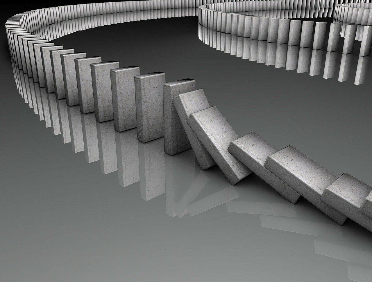
If you line up any number of dominoes in a row, and knock the first one over, then all the dominoes will fall.

Domino principle - infinite version

If you line up an infinite row of dominoes, one domino for each natural number, and you knock the first one over, then all the dominoes will fall.

2. Method of Minimum Counter-Example

Proposition (Prime factorization)

Every natural number greater than $1$ can be factored into primes.

General idea of method of minimum counter-example

Set up a proof by contradiction.
Let $m$ be the minimum number such that $S_m$ is not true.
Show that $S_k$ is not true for $k < m$ , which is the desired contradiction.

3. Invariant Induction

Proposition (Parity of handshakes)

At any party, at any point in time, define a person’s parity as odd or even according to the number of hands they have shaken. Then the number of people with odd parity must be even.

General idea of invariant induction

We have a time-varying world state: $W_0, W_1, W_2, \ldots$ .
The goal is to prove that some statement $S$ is true for all world states.
Argue:
- Statement $S$ is true for $W_0$ .
- If $S$ is true for $W_k$ , then it remains true for $W_{k+1}$ .

4. Structural Induction

Definition (String - recursive definition)

Fix some finite set of symbols $\Sigma$ . We define a string over $\Sigma$ recursively as follows.

Base case: The empty sequence, denoted $\epsilon$ , is a string.
Recursive rule: If $x$ is a string and $a \in \Sigma$ , then $ax$ is a string.

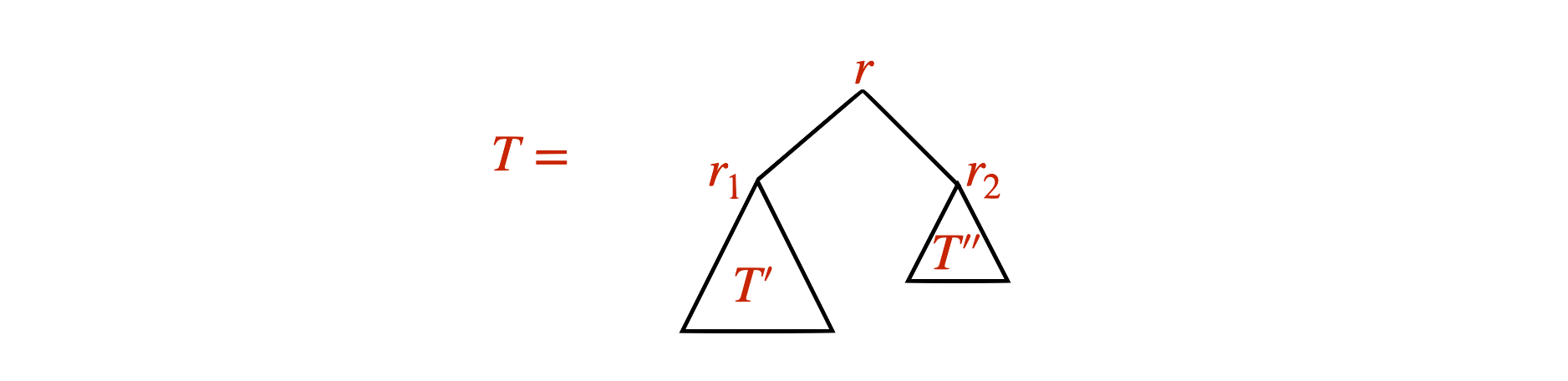
Definition (Binary tree - recursive definition)

We define a binary tree recursively as follows.

Base case: A single node $r$ is a binary tree with root $r$ .
Recursive rule: If $T'$ and $T''$ are binary trees with roots $r_1$ and $r_2$ , then $T$ , which has a node $r$ adjacent to $r_1$ and $r_2$ is a binary tree with root $r$ .

Proposition (Internal nodes vs leaves in binary trees)

Let $T$ be a binary tree. Let $L_T$ be the number of leaves in $T$ and let $I_T$ be the number of internal nodes in $T$ . Then $L_T = I_T + 1$ .

General idea of structural induction

You have a recursively defined set of objects, and you want to prove a statement $S$ about those objects.
Check that $S$ is true for the base case(s) of the recursive definition.
Prove $S$ holds for “new” objects created by the recursive rule, assuming it holds for “old” objects used in the recursive rule.

Some sketch of a “proof”

We prove statement $S$ by induction on the height of a tree. Let’s first check the base case... and it is true.

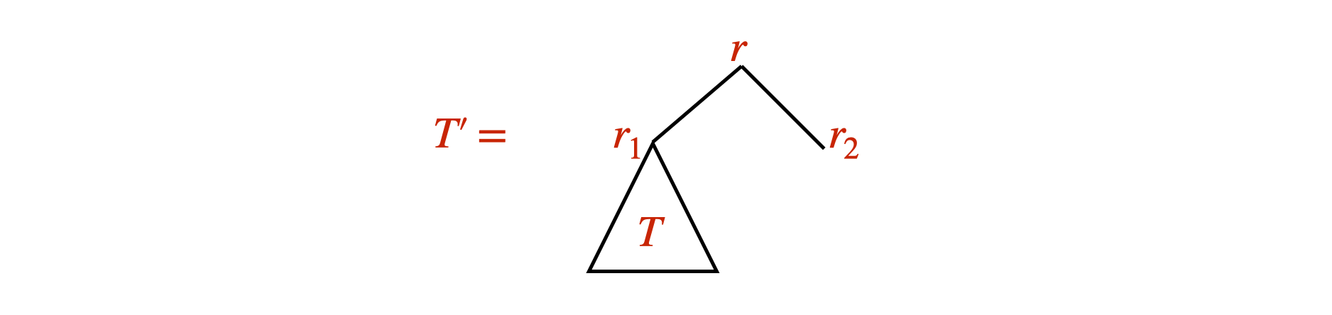
For the induction step, take an arbitrary binary tree $T$ of height $h$ . Let $T'$ be the following tree of height $h+1$ :

[Some argument showing why $S$ is true for $T'$ ] Therefore we are done.

Exercise (Recursively defined language)

Let $L$ be a set of binary strings (i.e. strings over $\Sigma = \{{\texttt{0}}, {\texttt{1}}\}$ ) defined recursively as follows:

(base case) the empty string, $\epsilon$ , is in $L$ ;
(recursive rule) if $x, y \in L$ , then ${\texttt{0}}x{\texttt{1}}y{\texttt{0}} \in L$ .

This means that every string in $L$ is derived starting from the base case, and applying the recursive rule a finite number of times. Show that for any string $w \in L$ , the number of ${\texttt{0}}$ ’s in $w$ is exactly twice the number of ${\texttt{1}}$ ’s in $w$ .

Important Note (On structural induction proof write-up)

In an induction argument on recursively defined objects, if you say that you will use structural induction, then the assumption is that the parameter being inducted on is the minimum number of applications of the recursive rules needed to create an object. And in this case, explicitly stating the parameter being inducted on, or the induction hypothesis, is not needed.

Encodings and Problems

1. Alphabets and Strings

Definition (Alphabet, symbol/character)

An alphabet is a non-empty, finite set, and is usually denoted by $\Sigma$ . The elements of $\Sigma$ are called symbols or characters.

Definition (String/word, empty string)

Given an alphabet $\Sigma$ , a string (or word) over $\Sigma$ is a (possibly infinite) sequence of symbols, written as $a_1a_2a_3\ldots$ , where each $a_i \in \Sigma$ . The string with no symbols is called the empty string and is denoted by $\epsilon$ .

Remark (Strings and quotation marks)

In our notation of a string, we do not use quotation marks. For instance, we write ${\texttt{1010}}$ rather than “ ${\texttt{1010}}$ ”, even though the latter notation using the quotation marks is the standard one in many programming languages. Occasionally, however, we may use quotation marks to distinguish a string like “ ${\texttt{1010}}$ ” from another type of object with the representation $1010$ (e.g. the binary number $1010$ ).

Definition (Length of a string)

The length of a string $w$ , denoted $|w|$ , is the number of symbols in $w$ . If $w$ has an infinite number of symbols, then the length is undefined.

Definition (Star operation on alphabets)

Let $\Sigma$ be an alphabet. We denote by $\Sigma^*$ the set of all strings over $\Sigma$ consisting of finitely many symbols. Equivalently, using set notation, $\Sigma^* = \{a_1a_2\ldots a_n : \text{ $n \in \mathbb N$, and $a_i \in \Sigma$ for all $i$}\}.$

Note (Finite vs infinite strings)

We will use the words “string” and “word” to refer to a finite-length string/word. When we want to talk about infinite-length strings, we will explicitly use the word “infinite”.

Note (Size of

\Sigma^*

)

By Definition (Alphabet, symbol/character), an alphabet $\Sigma$ cannot be the empty set. This implies that $\Sigma^*$ is an infinite set since there are infinitely many strings of finite length over a non-empty $\Sigma$ . We will later see that $\Sigma^*$ is always countably infinite.

Definition (Reversal of a string)

The reversal of a string $w = a_1a_2\ldots a_n$ , denoted $w^R$ , is the string $w^R = a_na_{n-1}\ldots a_1$ .

Definition (Concatenation of strings)

The concatenation of strings $u$ and $v$ in $\Sigma^*$ , denoted by $uv$ or $u \cdot v$ , is the string obtained by joining together $u$ and $v$ .

Definition (Powers of a string)

For $n \in \mathbb N$ , the $n$ ’th power of a string $u$ , denoted by $u^n$ , is the word obtained by concatenating $u$ with itself $n$ times.

Definition (Substring)

We say that a string $u$ is a substring of string $w$ if $w = xuy$ for some strings $x$ and $y$ .

Definition (Prefix, suffix)

For strings $x$ and $y$ , we say that $y$ is a prefix of $x$ if there exists a string $z$ such that $x = yz$ . If $z \neq \epsilon$ , then $y$ is a proper prefix of $x$ .

We say that $y$ is a suffix of $x$ if there exists a string $z$ such that $x = zy$ . If $z \neq \epsilon$ , then $y$ is a proper suffix of $x$ .

2. Encodings

Definition (Encoding elements of a set)

Let $A$ be a set and let $\Sigma$ be an alphabet. An encoding of the elements of $A$ , using $\Sigma$ , is an injective function $\text{Enc}: A \to \Sigma^*$ . We denote the encoding of $a \in A$ by $\left \langle a \right\rangle$ .

If $w \in \Sigma^*$ is such that there is some $a \in A$ with $w = \left \langle a \right\rangle$ , then we say $w$ is a valid encoding of an element in $A$ .

A set that can be encoded is called encodable.

Exercise (Unary encoding of integers)

Describe an encoding of $\mathbb Z$ using the alphabet $\Sigma = \{{\texttt{1}}\}$ .

3. Computational Problems

Definition (Function problem)

Let $\Sigma$ be an alphabet. Any function $f: \Sigma^* \to \Sigma^*$ is called a function problem over the alphabet $\Sigma$ .

Important Note (Function problem as mapping instances to solutions)

A function problem is often derived from a function $g: I \to S$ , where $I$ is a set of objects called instances and $S$ is a set of objects called solutions. The derivation is done through encodings $\text{Enc}: I \to \Sigma^*$ and $\text{Enc}': S \to \Sigma^*$ . With these encodings, we can create the function problem $f : \Sigma^* \to \Sigma^*$ . In particular, if $w = \left \langle x \right\rangle$ for some $x \in I$ , then we define $f(w)$ to be $\text{Enc}'(g(x))$ .

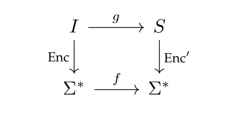
One thing we have to be careful about is defining $f(w)$ for a word $w \in \Sigma^*$ that does not correspond to an encoding of an object in $I$ (such a word does not correspond to an instance of the function problem). To handle this, we can identify one of the strings in $\Sigma^*$ as an error string and define $f(w)$ to be that string.

Definition (Decision problem)

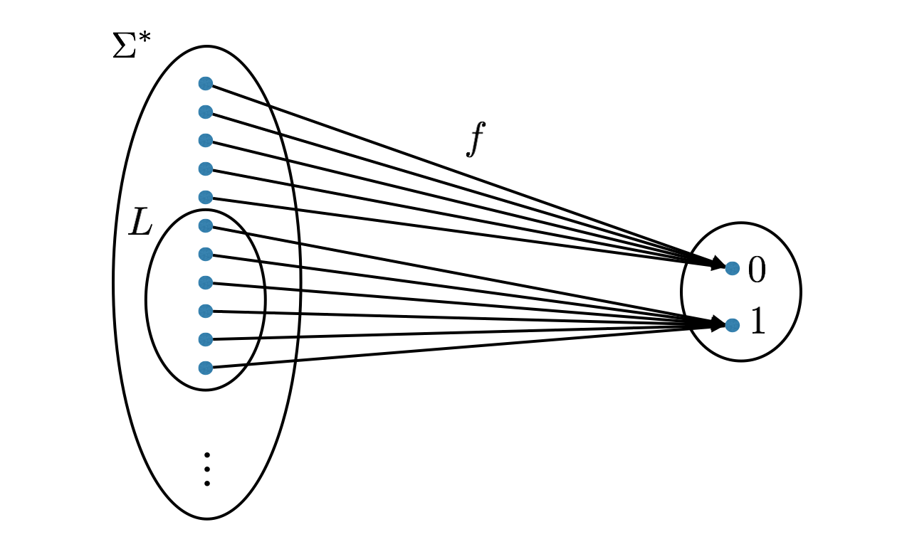
Let $\Sigma$ be an alphabet. Any function $f: \Sigma^* \to \{0,1\}$ is called a decision problem over the alphabet $\Sigma$ . The co-domain of the function is not important as long as it has two elements. One can think of the co-domain as $\{\text{No}, \text{Yes}\},$ $\{\text{False}, \text{True}\}$ or $\{ \text{Reject}, \text{Accept}\}$ .

Note (Decision problem as mapping instances to

0

1

As with a function problem, a decision problem is often derived from a function $g: I \to \{0,1\}$ , where $I$ is a set of instances. The derivation is done through an encoding $\text{Enc}: I \to \Sigma^*$ , which allows us to define the decision problem $f: \Sigma^* \to \{0,1\}$ . Any word $w \in \Sigma^*$ that does not correspond to an encoding of an instance is mapped to $0$ by $f$ .

Instances that map to $1$ are often called yes-instances and instances that map to $0$ are often called no-instances.

4. Decision Problems as Languages

Definition (Language)

Any (possibly infinite) subset $L \subseteq \Sigma^*$ is called a language over the alphabet $\Sigma$ .

Note (Size of a language)

Since a language is a set, the size of a language refers to the size of that set. A language can have finite or infinite size. This is not in conflict with the fact that every language consists of finite-length strings.

Remark (

\{\epsilon\}

\varnothing

)

The language $\{\epsilon\}$ is not the same language as $\varnothing$ . The former has size $1$ whereas the latter has size $0$ .

Important Note (Correspondence between decision problems and languages)

There is a one-to-one correspondence between decision problems and languages. Let $f:\Sigma^* \to \{0,1\}$ be some decision problem. Now define $L \subseteq \Sigma^*$ to be the set of all words in $\Sigma^*$ that $f$ maps to 1. This $L$ is the language corresponding to the decision problem $f$ . Similarly, if you take any language $L \subseteq \Sigma^*$ , we can define the corresponding decision problem $f:\Sigma^* \to \{0,1\}$ as $f(w) = 1$ if and only if $w \in L$ . We consider the set of languages and the set of decision problems to be the same set of objects.

It is important to get used to this correspondence since we will often switch between talking about languages and talking about decision problems without explicit notice.

Remark (The default alphabet)

When talking about decision/function problems or languages, if the alphabet is not specified, it is assumed to be the binary alphabet $\Sigma = \{{\texttt{0}}, {\texttt{1}}\}$ .

Remark (Why languages?)

You may be wondering why we make the definition of a language rather than always viewing a decision problem as a function from $\Sigma^*$ to $\{0,1\}$ . The reason is that some operations and notation are more conveniently expressed using sets rather than functions, and therefore in certain situations, it can be nicer to think of decision problems as sets.

5. Language Operations

Definition (Reversal of a language)

The reversal of a language $L \subseteq \Sigma^*$ , denoted $L^R$ , is the language $L^R = \{w^R \in \Sigma^* : w \in L\}.$

Definition (Concatenation of languages)

The concatenation of languages $L_1, L_2 \subseteq \Sigma^*$ , denoted $L_1L_2$ or $L_1 \cdot L_2$ , is the language $L_1L_2 = \{uv \in \Sigma^* : u \in L_1, v \in L_2\}.$

Definition (Powers of a language)

For $n \in \mathbb N$ , the $n$ ’th power of a language $L \subseteq \Sigma^*$ , denoted $L^n$ , is the language obtained by concatenating $L$ with itself $n$ times, that is, $L^n = \underbrace{L \cdot L \cdot L \cdots L}_{n \text{ times}}.$ Equivalently, $L^n = \{u_1u_2\cdots u_n \in \Sigma^* : u_i \in L \text{ for all } i \in \{1,2,\ldots,n\}\}.$

Definition (Star operation on a language)

The star of a language $L \subseteq \Sigma^*$ , denoted $L^*$ , is the language $L^* = \bigcup_{n \in \mathbb N} L^n.$ Equivalently, $L^* = \{u_1u_2\cdots u_n \in \Sigma^* : n \in \mathbb N, u_i \in L \text{ for all } i \in \{1,2,\ldots,n\}\}.$ Note that we always have $\epsilon\in L^*$ . Sometimes we may prefer to not include $\epsilon$ by default, so we define $L^+ = \bigcup_{n \in \mathbb N^+} L^n.$

Exercise (Can you distribute star over intersection?)

Prove or disprove: If $L_1, L_2 \subseteq \{{\texttt{a}},{\texttt{b}}\}^*$ are languages, then $(L_1 \cap L_2)^* = L_1^* \cap L_2^*$ .

Exercise (Can you distribute concatenation over union and intersection?)

Prove or disprove the following:

If $A, B, C \subseteq \{{\texttt{a}},{\texttt{b}}\}^*$ are languages, then $A(B \cup C) = AB \cup AC$ .
If $A, B, C \subseteq \{{\texttt{a}},{\texttt{b}}\}^*$ are languages, then $A(B \cap C) = AB \cap AC$ .

Exercise (Can you interchange star and reversal?)

Is it true that for any language $L$ , $(L^*)^R = (L^R)^*$ ? Prove your answer.

Exercise (Is single star equivalent to double star?)

Prove or disprove: For any language $L$ , $L^* = (L^*)^*$ .

Definition (Set of all languages)

We denote by $\mathsf{ALL}$ the set of all languages (over the default alphabet $\Sigma = \{{\texttt{0}}, {\texttt{1}}\}$ ).

6. Check Your Understanding

Problem

Given an alphabet $\Sigma$ , what is the definition of $\Sigma^*$ ?
What is the definition of a language?
Is $\varnothing$ a language? If it is, what is the decision problem corresponding to it?
Is $\Sigma^*$ a language? If it is, what is the decision problem corresponding to it?
Given two languages $L_1$ and $L_2$ , what are the definitions of $L_1L_2$ and $L_1^*$ ?
True or false: The language $\{{\texttt{011}}, {\texttt{101}}, {\texttt{110}}\}^*$ is the set of all binary strings containing twice as many ${\texttt{1}}$ ’s as ${\texttt{0}}$ ’s.
True or false: The set $\{\varnothing\}$ is a language, where $\varnothing$ denotes the empty set.
True or false: An infinite language must contain infinite-length strings.
True or false: A language can contain infinite-length strings.
Define finite languages $L_1$ and $L_2$ such that $|L_1L_2| < |L_1||L_2|$ .
Define finite languages $L_1$ and $L_2$ such that $|L_1L_2| = |L_1||L_2|$ .
True or false: For any language $L$ and any $n \in \mathbb N$ , we have $L^n \subseteq L^{n+1}$ .
True or false: For any language $L$ and any $n \in \mathbb N$ , we have $L^n \subseteq L^*$ .
Let $\Sigma$ be an alphabet. For which languages $L \subseteq \Sigma^*$ is it true that $L\cdot L$ is infinite?
Let $\Sigma$ be an alphabet. For which languages $L \subseteq \Sigma^*$ is it true that $L^*$ is infinite?
What is the definition of an encodable set? Which sets are encodable? How do we deal with sets that are not encodable?
What is the motivation behind defining an encoding as a mapping to finite-length strings as opposed to both finite and infinite-length strings?
What is the definition of a function problem? Give one example of a function problem.
What is the definition of a decision problem? Give one example of a decision problem.
Briefly explain the correspondence between decision problems and languages.
Write down the primality testing decision problem as a language.
Why do we focus on decision problems in theoretical computer science?

7. High-Order Bits

Important Note

Here are the important things to keep in mind from this chapter.

All the definitions and the notation introduced in this are fundamental, and we will use them liberally without reminders. As we move to more advanced topics, it is important that the definitions in this chapter do not add to the mental burden and make things overwhelming for you. Even when you are totally comfortable with the definitions, we will be covering concepts that are quite challenging. Therefore, you want to be able to spend all your mental energy on digesting the new material without getting confused by the definitions and terminology from previous chapters. If you invest the time to really understanding the definitions now, it will save you time later.
There is only one data type in theoretical computer science: strings. Every other type of data (e.g. numbers, images, graphs, videos) can be encoded with strings. Algorithms/computers work with these encodings.
A decision problem is a special kind of function problem. In a decision problem, for every possible input, the output is either True or False. Our focus for the next few chapters will be on decision problems.
There is a one-to-one correspondence between decision problems and languages. It is important to be able to easily switch between a language and the corresponding decision problem in your mind.

Deterministic Finite Automata

1. Basic Definitions

Computational Model

Anything that processes information can be called a computer. However, there can be restrictions on how the information can be processed (either universal restrictions imposed by, say, the laws of physics, or restrictions imposed by the particular setting we are interested in).

A computational model is a set of allowed rules for information processing. Given a computational model, we can talk about the computers (or machines) allowed by the computational model. A computer is a specific instantiation of the computational model, or in other words, it is a specific collection of information processing rules allowed by the computational model.

Note that even though the terms “computer” and “machine” suggest a physical device, in this course we are not interested in physical representations that realize computers, but rather in the mathematical representations. The term algorithm is synonymous to computer (and machine) and makes it more clear that we are not necessarily talking about a physical device.

Definition (Deterministic Finite Automaton (DFA))

A deterministic finite automaton (DFA) $M$ is a $5$ -tuple $M = (Q, \Sigma, \delta, q_0, F),$ where

$Q$ is a non-empty finite set (which we refer to as the set of states of the DFA);
$\Sigma$ is a non-empty finite set (which we refer to as the alphabet of the DFA);
$\delta$ is a function of the form $\delta: Q \times \Sigma \to Q$ (which we refer to as the transition function of the DFA);
$q_0 \in Q$ is an element of $Q$ (which we refer to as the start state of the DFA);
$F \subseteq Q$ is a subset of $Q$ (which we refer to as the set of accepting states of the DFA).

Note (State diagram of a DFA)

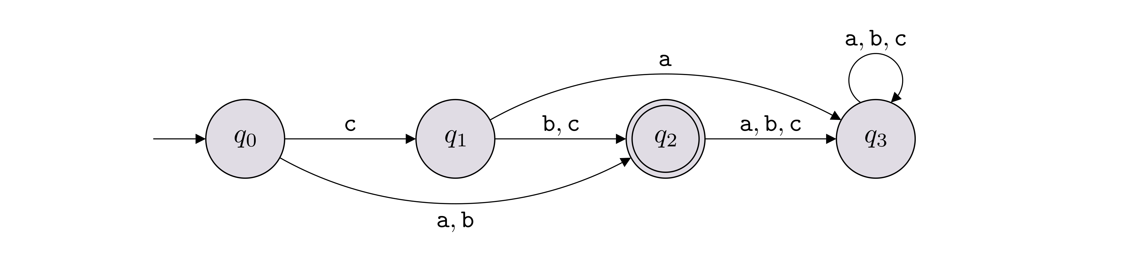
It is very common to represent a DFA with a state diagram. Below is an example of how we draw a state diagram of a DFA:

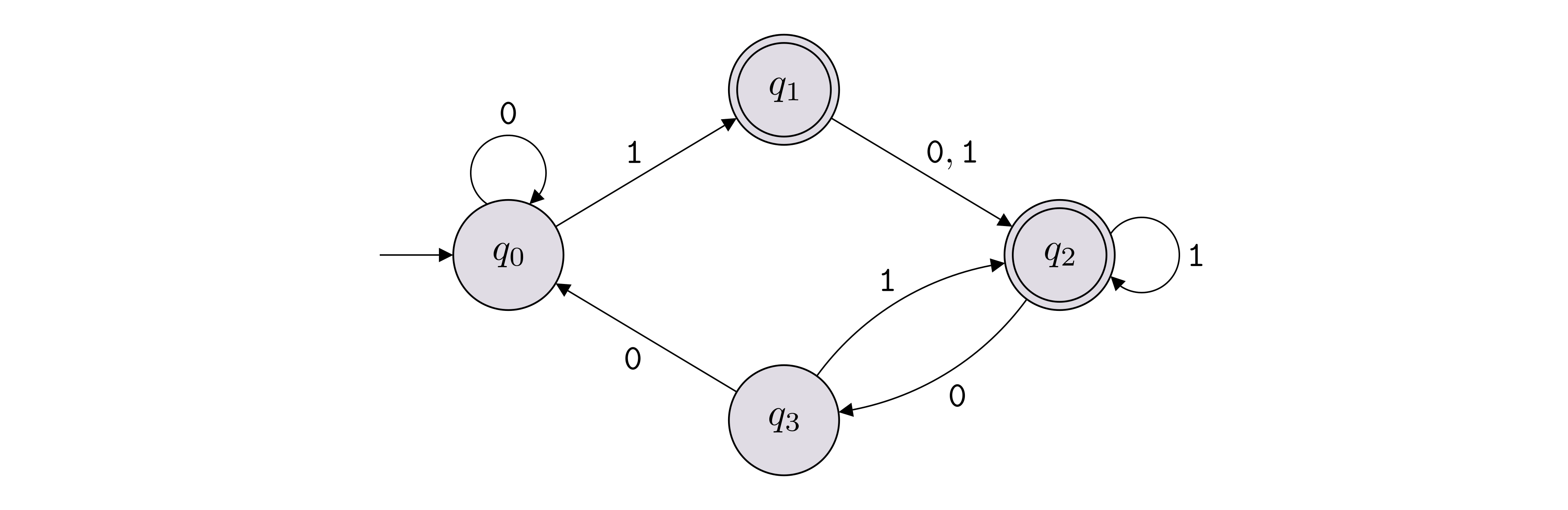
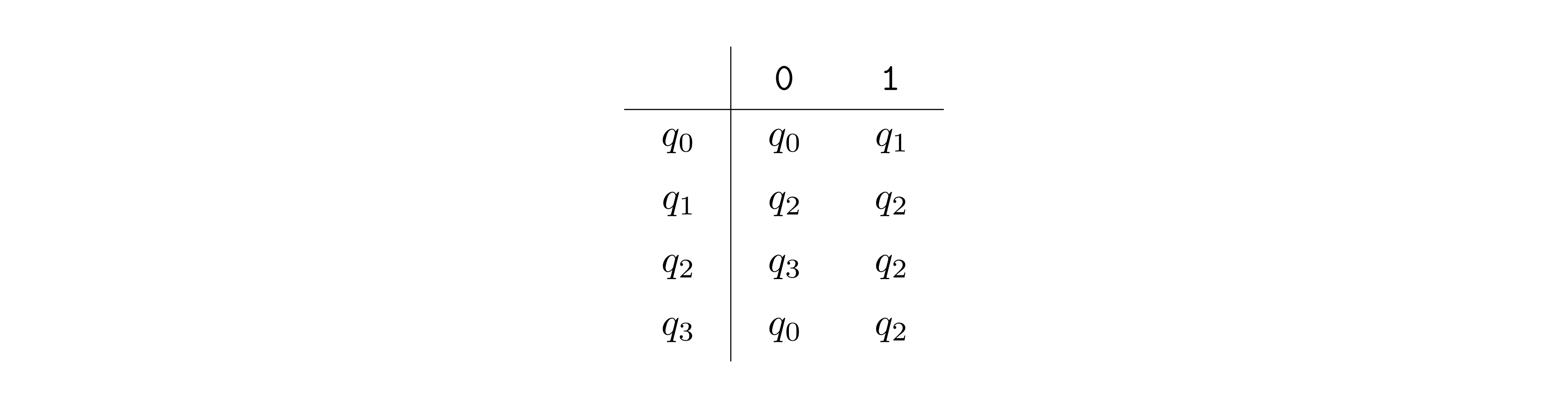
In this example, $\Sigma = \{{\texttt{0}},{\texttt{1}}\}$ , $Q = \{q_0,q_1,q_2,q_3\}$ , $F = \{q_1,q_2\}$ . The labeled arrows between the states encode the transition function $\delta$ , which can also be represented with a table as shown below (row $q_i \in Q$ and column $b \in \Sigma$ contains $\delta(q_i, b)$ ).

The start state is labeled with $q_0$ , but if another label is used, we can identify the start state in the state diagram by identifying the state with an arrow that does not originate from another state and goes into that state.

Remark (The labels of DFA components)

In the definition above, we used the labels $Q, \Sigma, \delta, q_0, F$ . One can of course use other labels when defining a DFA as long as it is clear what each label represents.

Remark (Equivalence of DFAs)

We’ll consider two DFAs to be equivalent/same if they are the same machine up to renaming the elements of the sets $Q$ and $\Sigma$ . For instance, the two DFAs below are considered to be the same even though they have different labels on the states and use different alphabets.

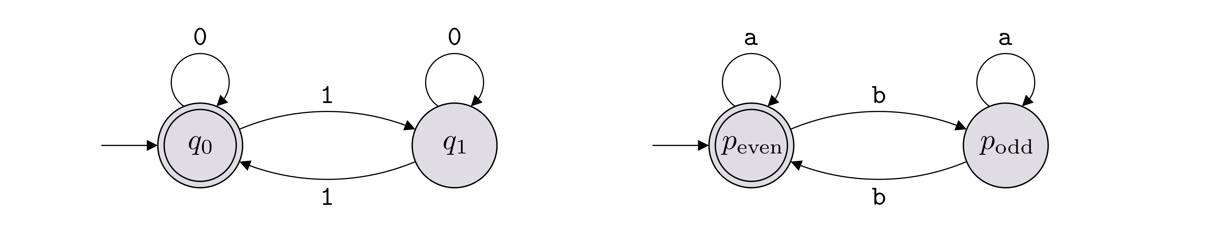
The flexibility with the choice of labels allows us to be more descriptive when we define a DFA. For instance, we can give labels to the states that communicate the “purpose” or “role” of each state.

Definition (Computation path for a DFA)

Let $M = (Q, \Sigma, \delta, q_0, F)$ be a DFA and let $w = w_1w_2 \cdots w_n$ be a string over an alphabet $\Sigma$ (so $w_i \in \Sigma$ for each $i \in \{1,2,\ldots,n\}$ ). The computation path of $M$ with respect to $w$ is a specific sequence of states $r_0, r_1, r_2, \ldots , r_n$ (where each $r_i \in Q$ ). We’ll often write this sequence as follows.

	$w_1$	$w_2$	$\ldots$	$w_n$
$r_0$	$r_1$	$r_2$	$\ldots$	$r_n$

These states correspond to the states reached when the DFA reads the input $w$ one character at a time. This means $r_0 = q_0$ , and $\forall i \in \{1,2,\ldots,n\}, \quad \delta(r_{i-1},w_i) = r_i.$ An accepting computation path is such that $r_n \in F$ , and a rejecting computation path is such that $r_n \not\in F$ .

We say that $M$ accepts a string $w \in \Sigma^*$ (or “ $M(w)$ accepts”, or “ $M(w) = 1$ ”) if the computation path of $M$ with respect to $w$ is an accepting computation path. Otherwise, we say that $M$ rejects the string $w$ (or “ $M(w)$ rejects”, or “ $M(w) = 0$ ”).

Note (Extended transition function)

Let $M = (Q, \Sigma, \delta, q_0, F)$ be a DFA. The transition function $\delta : Q \times \Sigma \to Q$ extends to $\delta^* : Q \times \Sigma^* \to Q$ , where $\delta^*(q, w)$ is defined as the state we end up in if we start at $q$ and read the string $w = w_1 \ldots w_n$ . Or in other words, $\delta^*(q, w) = \delta(\ldots\delta(\delta(\delta(q,w_1),w_2),w_3)\ldots, w_n).$ The star in the notation can be dropped and $\delta$ can be overloaded to represent both a function $\delta : Q \times \Sigma \to Q$ and a function $\delta : Q \times \Sigma^* \to Q$ . Using this notation, a word $w$ is accepted by the DFA $M$ if $\delta(q_0, w) \in F$ .

Definition (DFA solving a decision problem or a language)

Let $f: \Sigma^* \to \{0,1\}$ be a decision problem and let $M$ be a DFA over the same alphabet. We say that $M$ solves (or decides, or computes) $f$ if the input/output behavior of $M$ matches $f$ exactly, in the following sense: for all $w \in \Sigma^*$ , $M(w) = f(w)$ .

If $L$ is the language corresponding to $f$ , the above definition is equivalent to saying that $M$ solves (or decides, or computes) $L$ if the following holds:

if $w \in L$ , then $M$ accepts $w$ (i.e. $M(w) = 1$ );
if $w \not \in L$ , then $M$ rejects $w$ (i.e. $M(w) = 0$ ).

Note (Uniqueness of the language of a DFA)

For a DFA $M$ , there is a unique language $L$ that $M$ solves. This language is often denoted by $L(M)$ and is referred to as the language of $M$ . Note that $L(M) = \{w \in \Sigma^* : \text{$M$ accepts $w$}\}.$

Exercise (Describe the language of a DFA)

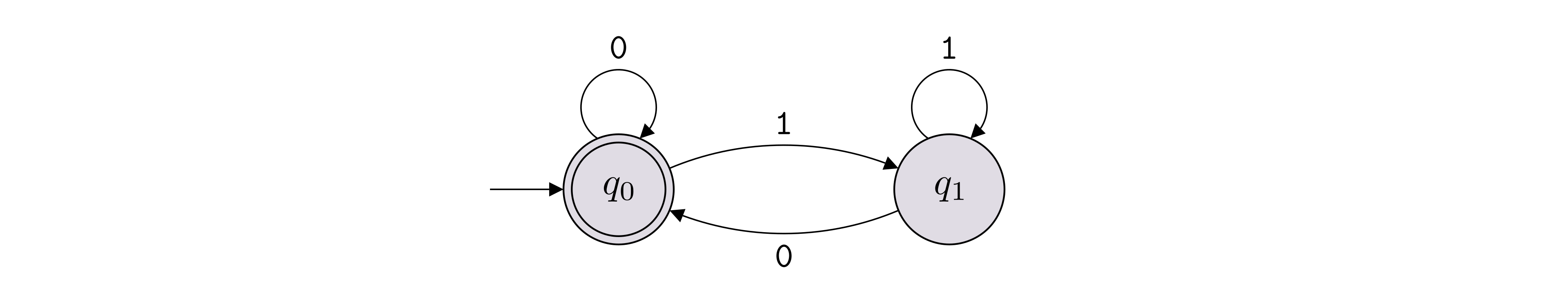
For each DFA $M$ below, define $L(M)$ .

Exercise (Draw DFAs)

For each language below (over the alphabet $\Sigma = \{{\texttt{0}},{\texttt{1}}\}$ ), draw a DFA solving it.

$\{{\texttt{101}}, {\texttt{110}}\}$
$\{{\texttt{0}},{\texttt{1}}\}^* \setminus \{{\texttt{101}}, {\texttt{110}}\}$
$\{x \in \{{\texttt{0}},{\texttt{1}}\}^* : \text{$x$ starts and ends with the same bit}\}$
$\{{\texttt{110}}\}^* = \{\epsilon, {\texttt{110}}, {\texttt{110110}}, {\texttt{110110110}}, \ldots\}$
$\{x \in \{{\texttt{0}},{\texttt{1}}\}^*: \text{$x$ contains ${\texttt{110}}$ as a substring}\}$

Exercise (Finite languages can be solved by DFAs)

Let $L$ be a finite language, i.e., it contains a finite number of words. At a high level, describe why there is a DFA solving $L$ .

Definition (Regular language)

A language $L \subseteq \Sigma^*$ is called a regular language if there is a deterministic finite automaton $M$ that solves $L$ .

Exercise (Equal number of

{\texttt{01}}

’s and

{\texttt{10}}

’s)

Let $\Sigma = \{{\texttt{0}},{\texttt{1}}\}$ . Is the following language regular? $L = \{w \in \{{\texttt{0}},{\texttt{1}}\}^* : w \text{ has an equal number of occurrences of ${\texttt{01}}$ and ${\texttt{10}}$ as substrings}\}$

Definition (Complexity class

\mathsf{REG}

)

We denote by $\mathsf{REG}$ the set of all regular languages (over the default alphabet $\Sigma = \{{\texttt{0}}, {\texttt{1}}\}$ ).

2. Non-Regular Languages

Theorem (

{\texttt{0}}^n {\texttt{1}}^n

is not regular)

Let $\Sigma = \{{\texttt{0}},{\texttt{1}}\}$ . The language $L = \{{\texttt{0}}^n {\texttt{1}}^n: n \in \mathbb N\}$ is not regular.

Exercise (Would any set of pigeons work?)

In the proof of the above theorem, we defined the set $P = \{{\texttt{0}}^n : n \in \{0,1,\ldots,k\}\}$ and then applied the pigeonhole principle. Explain why picking the following sets would not have worked in that proof.

$P = \{{\texttt{1}}^n : n \in \{1,2,\ldots,k+1\}\}$
$P = \{{\texttt{1}}, {\texttt{11}}, {\texttt{000}}, {\texttt{0000}}, {\texttt{00000}}, \ldots, {\texttt{0}}^{k+1}\}$

Exercise (

{\texttt{c}}^{251}{\texttt{a}}^n{\texttt{b}}^{2n}

is not regular)

Let $\Sigma = \{{\texttt{a}},{\texttt{b}},{\texttt{c}}\}$ . Prove that $L = \{{\texttt{c}}^{251} {\texttt{a}}^n {\texttt{b}}^{2n}: n \in \mathbb N\}$ is not regular.

Exercise (A fooling pigeon set)

In Exercise (Would any set of pigeons work?) we saw that the “pigeon set” that we use to apply the pigeonhole principle must be chosen carefully. We’ll call a pigeon set a fooling pigeon set if it is a pigeon set that “works”. That is, given a DFA with $k$ states that is assumed to solve a non-regular $L$ , a fooling pigeon set of size $k+1$ allows us to carry out the contradiction proof, and conclude that $L$ is non-regular. Identify the property that a fooling pigeon set should have.

Theorem (A unary non-regular language)

Let $\Sigma = \{{\texttt{a}}\}$ . The language $L = \{{\texttt{a}}^{2^n}: n \in \mathbb N\}$ is not regular.

Note (Lower-bounding the number of states)

In the next exercise, we’ll write the proof in a slightly different way to offer a slightly different perspective. In particular, we’ll phrase the proof such that the goal is to show no DFA solving $L$ can have a finite number of states. This is done by identifying an infinite set of strings that all must end up in a different state (this is the fooling pigeon set that we defined in Exercise (A fooling pigeon set)). Once you have a set of strings $S$ such that every string in $S$ must end up in a different state, we can conclude any DFA solving the language must have at least $|S|$ states.

This slight change in phrasing of the non-regularity proof makes it clear that even if $L$ is regular, the technique can be used to prove a lower bound on the number of states of any DFA solving $L$ .

Exercise (

{\texttt{a}}^n{\texttt{b}}^n{\texttt{c}}^n

is not regular)

Let $\Sigma = \{{\texttt{a}},{\texttt{b}},{\texttt{c}}\}$ . Prove that $L = \{{\texttt{a}}^n{\texttt{b}}^n{\texttt{c}}^n: n \in \mathbb N\}$ is not regular.

3. Closure Properties of Regular Languages

Exercise (Are regular languages closed under complementation?)

Is it true that if $L$ is regular, then its complement $\Sigma^* \setminus L$ is also regular? In other words, are regular languages closed under the complementation operation?

Exercise (Are regular languages closed under subsets?)

Is it true that if $L \subseteq \Sigma^*$ is a regular language, then any $L' \subseteq L$ is also a regular language?

Theorem (Regular languages are closed under union)

Let $\Sigma$ be some finite alphabet. If $L_1 \subseteq \Sigma^*$ and $L_2 \subseteq \Sigma^*$ are regular languages, then the language $L_1 \cup L_2$ is also regular.

Corollary (Regular languages are closed under intersection)

Let $\Sigma$ be some finite alphabet. If $L_1 \subseteq \Sigma^*$ and $L_2 \subseteq \Sigma^*$ are regular languages, then the language $L_1 \cap L_2$ is also regular.

Exercise (Direct proof that regular languages are closed under difference)

Give a direct proof (without using the fact that regular languages are closed under complementation, union and intersection) that if $L_1$ and $L_2$ are regular languages, then $L_1 \setminus L_2$ is also regular.

Exercise (Finite vs infinite union)

Suppose $L_1, \ldots, L_k$ are all regular languages. Is it true that their union $\bigcup_{i=0}^k L_i$ must be a regular language?
Suppose $L_0, L_1, L_2, \ldots$ is an infinite sequence of regular languages. Is it true that their union $\bigcup_{i\geq 0} L_i$ must be a regular language?

Exercise (Union of non-regular languages)

Suppose $L_1$ and $L_2$ are not regular languages. Is it always true that $L_1 \cup L_2$ is not a regular language?

Exercise (Regularity of suffixes and prefixes)

Suppose $L \subseteq \Sigma^*$ is a regular language. Show that the following languages are also regular: $\begin{aligned} \text{SUFFIXES}(L) & = \{x \in \Sigma^* : \text{$yx \in L$ for some $y \in \Sigma^*$}\}, \\ \text{PREFIXES}(L) & = \{y \in \Sigma^* : \text{$yx \in L$ for some $x \in \Sigma^*$}\}.\end{aligned}$

Theorem (Regular languages are closed under concatenation)

If $L_1, L_2 \subseteq \Sigma^*$ are regular languages, then the language $L_1L_2$ is also regular.

Definition (Generalized transition function)

Let $M = (Q, \Sigma, \delta, q_0, F)$ be a DFA. We define the generalized transition function $\delta_\wp: \wp(Q) \times \Sigma \to \wp(Q)$ as follows. For $S \subseteq Q$ and $\sigma \in \Sigma$ , $\delta_{\wp}(S, \sigma) = \{\delta(q, \sigma) : q \in S\}.$

Exercise (Regular languages are closed under concatenation - another construction)

In the proof of Theorem (Regular languages are closed under concatenation), we defined the set of states for the DFA solving $L_1L_2$ as $Q'' = Q \times \wp(Q')$ . Construct a DFA for $L_1L_2$ in which $Q''$ is equal to $\wp(Q \cup Q')$ , i.e., specify how $\delta''$ , $q_0''$ and $F''$ should be defined with respect to $Q'' = \wp(Q \cup Q')$ . Proof of correctness is not required.

Exercise (Regular languages are closed under star - wrong proof)

Critique the following argument that claims to establish that regular languages are closed under the star operation, that is, if $L$ is a regular language, then so is $L^*$ .

Let $L$ be a regular language. We know that by definition $L^* = \bigcup_{n \in \mathbb N} L^n$ , where $L^n = \{u_1 u_2 \ldots u_n : u_i \in L \text{ for all $i$} \}.$ We know that for all $n$ , $L^n$ must be regular using Theorem (Regular languages are closed under concatenation). And since $L^n$ is regular for all $n$ , we know $L^*$ must be regular using Theorem (Regular languages are closed under union).

Exercise (Regular languages are closed under star - correct proof)

Show that regular languages are closed under the star operation as follows: First show that if $L$ is regular, then so is $L^+$ , which is defined as the union $L^+ = \bigcup_{n \in \mathbb N^+} L^n.$ For this part, given a DFA for $L$ , show how to construct a DFA for $L^+$ . A proof of correctness is not required. In order to conclude that $L^*$ is regular, observe that $L^* = L^+ \cup \{\epsilon\}$ , and use the fact that regular languages are closed under union.

4. Bonus: Non-Deterministic FA

5. Check Your Understanding

Problem

What are the $5$ components of a DFA?
Let $M$ be a DFA. What does $L(M)$ denote?
Draw a DFA solving $\varnothing$ . Draw a DFA solving $\Sigma^*$ .
True or false: Given a language $L$ , there is at most one DFA that solves it.
Fix some alphabet $\Sigma$ . How many DFAs are there with exactly one state?
True or false: For any DFA, all the states are “reachable”. That is, if $D = (Q, \Sigma, \delta, q_0, F)$ is a DFA and $q \in Q$ is one of its states, then there is a string $w \in \Sigma^*$ such that $\delta^*(q_0,w) = q$ .
What is the set of all possible inputs for a DFA $D = (Q, \Sigma, \delta, q_0, F)$ ?
Consider the set of all DFAs with $k$ states over the alphabet $\Sigma =\{{\texttt{a}}\}$ such that all states are reachable from $q_0$ . What is the cardinality of this set?
What is the definition of a regular language?
Describe the general strategy (the high level steps) for showing that a language is not regular.
Give $3$ examples of non-regular languages.
Let $L \subseteq \{{\texttt{a}}\}^*$ be a language consisting of all strings of ${\texttt{a}}$ ’s of odd length except length $251$ . Is $L$ regular?
Let $L$ be the set of all strings in $\{{\texttt{0}},{\texttt{1}}\}^*$ that contain at least $251$ ${\texttt{0}}$ ’s and at most $251$ ${\texttt{1}}$ ’s. Is $L$ regular?
Suppose you are given a regular language $L$ and you are asked to prove that any DFA solving $L$ must contain at least $k$ states (for some $k$ value given to you). What is a general proof strategy for establishing such a claim?
Let $M = (Q, \Sigma, \delta, q_0, F)$ be a DFA solving a language $L$ and let $M' = (Q', \Sigma, \delta', q'_0, F')$ be a DFA solving a language $L'$ . Describe the $5$ components of a DFA solving $L \cup L'$ .
True or false: Let $L_1 \oplus L_2$ denote the set of all words in either $L_1$ or $L_2$ , but not both. If $L_1$ and $L_2$ are regular, then so is $L_1 \oplus L_2$ .
True or false: For languages $L$ and $L'$ , if $L \subseteq L'$ and $L$ is non-regular, then $L'$ is non-regular.
True or false: If $L \subseteq \Sigma^*$ is non-regular, then $\overline{L} = \Sigma^* \setminus L$ is non-regular.
True or false: If $L_1, L_2 \subseteq \Sigma^*$ are non-regular languages, then so is $L_1 \cup L_2$ .
True or false: Let $L$ be a non-regular language. There exists $K \subset L$ , $K \neq L$ , such that $K$ is also non-regular.
By definition a DFA has finitely many states. What is the motivation/reason for this restriction?
Consider the following decision problem: Given as input a DFA, output True if and only if there exists some string $s \in \Sigma^*$ that the DFA accepts. Write the language corresponding to this decision problem using mathematical notation, and in particular, using set builder notation.

6. High-Order Bits

Important Note

Here are the important things to keep in mind from this chapter.

Given a DFA, describe in English the language that it solves.
Given the description of a regular language, come up with a DFA that solves it.
Given a non-regular language, prove that it is indeed non-regular. Make sure you are not just memorizing a template for these types of proofs, but that you understand all the details of the strategy being employed. Apply the Feynman technique and see if you can teach this kind of proof to someone else.
In proofs establishing a closure property of regular languages, you start with one or more DFAs, and you construct a new one from them. In order to build the new DFA successfully, you have to be comfortable with the 5-tuple notation of a DFA. The constructions can get notation-heavy (with power sets and Cartesian products), but getting comfortable with mathematical notation is one of our learning objectives.
With respect to closure properties of regular languages, prioritize having a very solid understanding of closure under the union operation before you move to the more complicated constructions for the concatenation operation and star operation.

Turing Machines

1. Turing Machines and Decidability

Definition (Turing machine)

A Turing machine (TM) $M$ is a 7-tuple $M = (Q, \Sigma, \Gamma, \delta, q_0, q_\text{acc}, q_\text{rej}),$ where

$Q$ is a non-empty finite set
(which we refer to as the set of states of the TM);
$\Sigma$ is a non-empty finite set that does not contain the blank symbol $\sqcup$
(which we refer to as the input alphabet of the TM);
$\Gamma$ is a finite set such that $\sqcup\in \Gamma$ and $\Sigma \subset \Gamma$
(which we refer to as the tape alphabet of the TM);
$\delta$ is a function of the form $\delta: Q \times \Gamma \to Q \times \Gamma \times \{\text{L}, \text{R}\}$
(which we refer to as the transition function of the TM);
$q_0 \in Q$ is an element of $Q$
(which we refer to as the initial state of the TM or the starting state of the TM);
$q_\text{acc}\in Q$ is an element of $Q$
(which we refer to as the accepting state of the TM);
$q_\text{rej}\in Q$ is an element of $Q$ such that $q_\text{rej}\neq q_\text{acc}$
(which we refer to as the rejecting state of the TM).

Note (State diagram of a TM)

Below is an example of a state diagram of a TM with $5$ states:

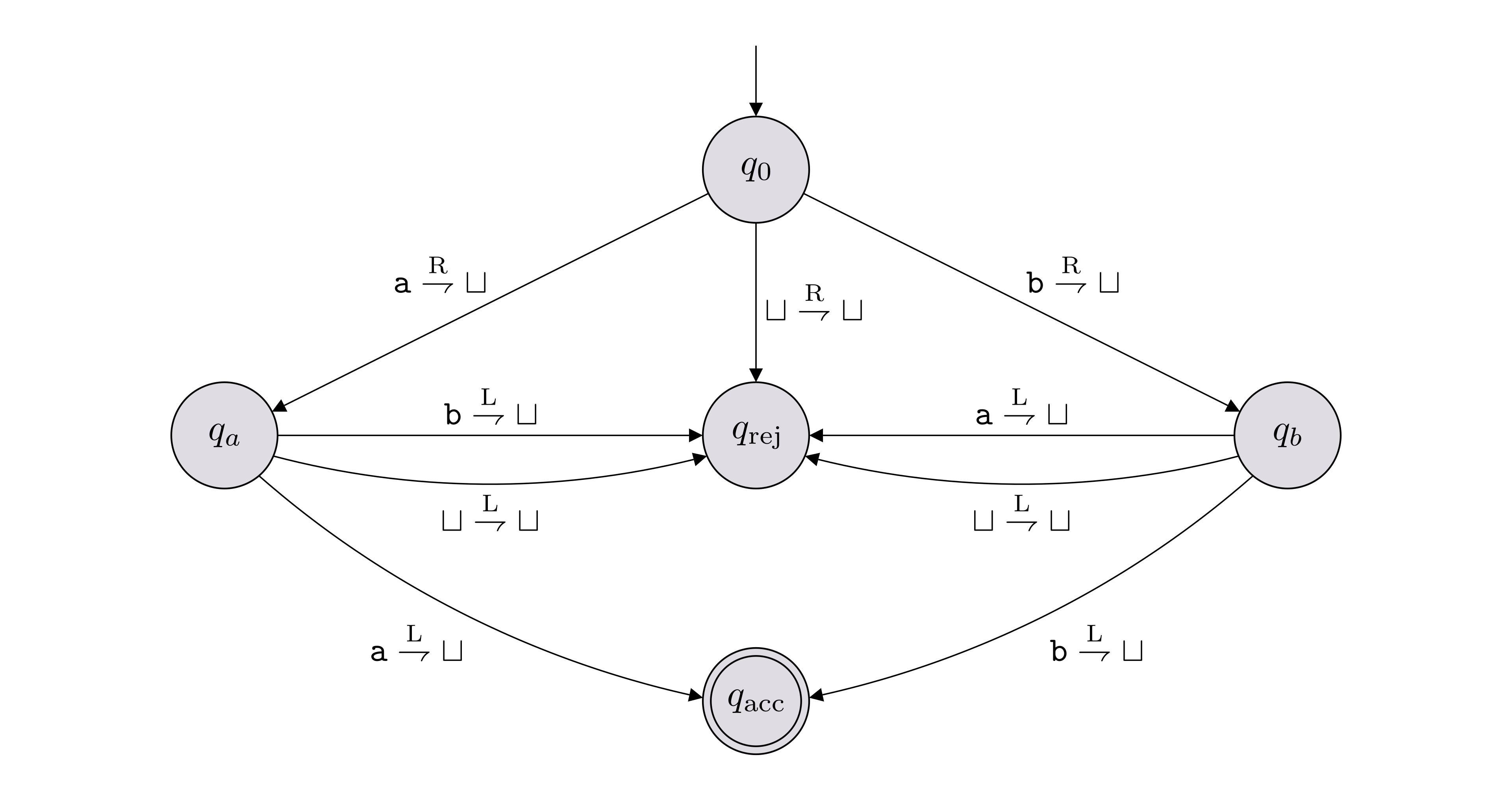
In this example, $\Sigma = \{{\texttt{a}},{\texttt{b}}\}$ , $\Gamma = \{{\texttt{a}},{\texttt{b}},\sqcup\}$ , $Q = \{q_0,q_a,q_b,q_\text{acc},q_\text{rej}\}$ . The labeled arrows between the states encode the transition function $\delta$ . As an example, the label on the arrow from $q_0$ to $q_a$ is ${\texttt{a}} \overset{\text{R}}{\rightharpoondown} \sqcup$ , which represents $\delta(q_0, {\texttt{a}}) = (q_a, \sqcup, \text{R})$

Important Note (A Turing machine uses a tape)

A Turing machine is always accompanied by a tape that is used as memory. The tape is just a sequence of cells that can hold any symbol from the tape alphabet. The tape can be defined so that it is infinite in two directions (so we could imagine indexing the cells using the integers $\mathbb Z$ ), or it could be infinite in one direction, to the right (so we could imagine indexing the cells using the natural numbers $\mathbb N$ ). The input to a Turing machine is always a string $w \in \Sigma^*$ . The string $w_1\ldots w_n \in \Sigma^*$ is put on the tape so that symbol $w_i$ is placed on the cell with index $i-1$ . We imagine that there is a tape head that initially points to index 0. The symbol that the tape head points to at a particular time is the symbol that the Turing machine reads. The tape head moves left or right according to the transition function of the Turing machine. These details are explained in lecture.

In these notes, we assume our tape is infinite in two directions.

Important Note (Turing machines can loop forever)

Given any DFA and any input string, the DFA always halts and makes a decision to either reject or accept the string. The same is not true for TMs and this is an important distinction between DFAs and TMs. It is possible that a TM does not make a decision when given an input string, and instead, loops forever. So given a TM $M$ and an input string $x$ , there are 3 options when we run $M$ on $x$ :

$M$ accepts $x$ (denoted $M(x) = 1$ );
$M$ rejects $x$ (denoted $M(x) = 0$ );
$M$ loops forever (denoted $M(x) = \infty$ ).

The formal definitions for these 3 cases is given below.

Definition (Computation path for a TM)

Let $M$ be a Turing machine where $Q$ is the set of states, $\sqcup$ is the blank symbol, and $\Gamma$ is the tape alphabet. To understand how $M$ ’s computation proceeds we generally need to keep track of three things: (i) the state $M$ is in; (ii) the contents of the tape; (iii) where the tape head is. These three things are collectively known as the “configuration” of the TM. More formally: a configuration for $M$ is defined to be a string $uqv \in (\Gamma \cup Q)^*$ , where $u, v \in \Gamma^*$ and $q \in Q$ . This represents that the tape has contents $\cdots \sqcup\sqcup\sqcup uv \sqcup\sqcup\sqcup\cdots$ , the head is pointing at the leftmost symbol of $v$ , and the state is $q$ . A configuration is an accepting configuration if $q$ is $M$ ’s accept state and it is a rejecting configuration if $q$ is $M$ ’s reject state.

Suppose that $M$ reaches a certain configuration $\alpha$ (which is not accepting or rejecting). Knowing just this configuration and $M$ ’s transition function $\delta$ , one can determine the configuration $\beta$ that $M$ will reach at the next step of the computation. (As an exercise, make this statement precise.) We write $\alpha \vdash_M \beta$ and say that “ $\alpha$ yields $\beta$ (in $M$ )”. If it is obvious what $M$ we’re talking about, we drop the subscript $M$ and just write $\alpha \vdash \beta$ .

Given an input $x \in \Sigma^*$ we say that $M(x)$ halts if there exists a sequence of configurations (called the computation path) $\alpha_0, \alpha_1, \dots, \alpha_{T}$ such that:

$\alpha_0 = q_0x$ , where $q_0$ is $M$ ’s initial state;
$\alpha_t \vdash_M \alpha_{t+1}$ for all $t = 0, 1, 2, \dots, T-1$ ;
$\alpha_T$ is either an accepting configuration (in which case we say $M(x)$ accepts) or a rejecting configuration (in which case we say $M(x)$ rejects).

Otherwise, we say $M(x)$ loops.

Exercise (Practice with configurations)

Let $M$ denote the Turing machine shown below, which has input alphabet $\Sigma = \{{\texttt{0}}\}$ and tape alphabet $\Gamma = \{{\texttt{0}},{\texttt{x}}, \sqcup\}$ .

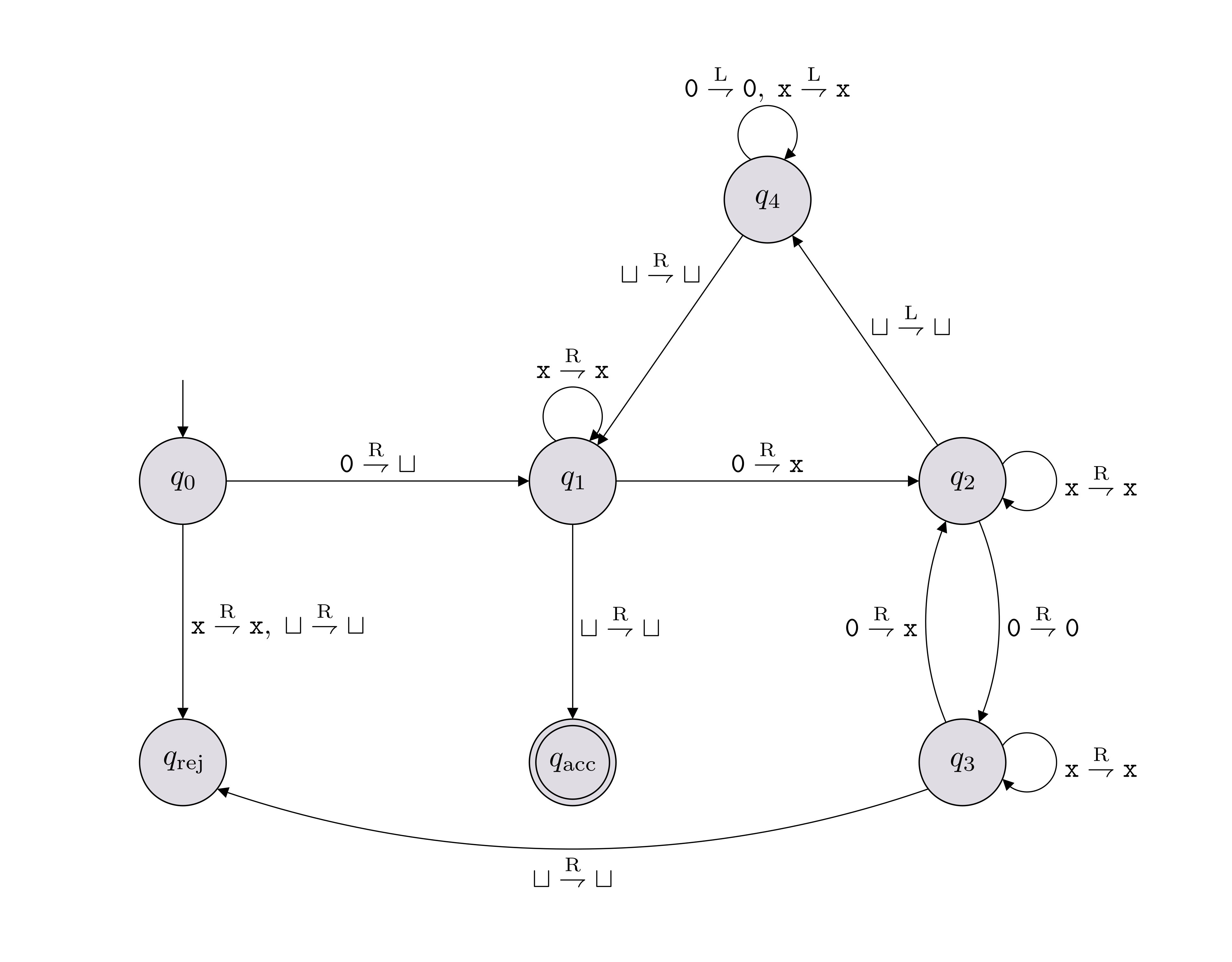
Write out the computation path $\alpha_0 \vdash_M \alpha_1 \vdash_M \cdots \vdash_M \alpha_T$ for $M({\texttt{0000}})$ and determine whether it accepts or rejects.

Definition (TM solving/deciding a language or decision problem)

Let $f: \Sigma^* \to \{0,1\}$ be a decision problem and let $M$ be a TM with input alphabet $\Sigma$ . We say that $M$ solves (or decides, or computes) $f$ if the input/output behavior of $M$ matches $f$ exactly, in the following sense: for all $w \in \Sigma^*$ , $M(w) = f(w)$ .

If $L$ is the language corresponding to $f$ , the above definition is equivalent to saying that $M$ solves (or decides, or computes) $L$ if the following holds:

if $w \in L$ , then $M$ accepts $w$ (i.e. $M(w) = 1$ );
if $w \not \in L$ , then $M$ rejects $w$ (i.e. $M(w) = 0$ ).

If $M$ solves a decision problem (language), $M$ must halt on all inputs. Such a TM is called a decider.

Note (Language of a TM)

The language of a TM $M$ is $L(M) = \{w \in \Sigma^* : \text{$M$ accepts $w$}\}.$ Given a TM $M$ , we cannot say that $M$ solves/decides $L(M)$ because $M$ may loop forever for inputs $w$ not in $L(M)$ . Only a decider TM can decide a language. And if $M$ is indeed a decider, then $L(M)$ is the unique language that $M$ solves/decides.

Exercise (A simple decidable language)

Give a description of the language decided by the TM shown in Note (State diagram of a TM).

Exercise (Drawing TM state diagrams)

For each language below, draw the state diagram of a TM that decides the language. You can use any finite tape alphabet $\Gamma$ containing the elements of $\Sigma$ and the symbol $\sqcup$ .

$L = \{{\texttt{0}}^n{\texttt{1}}^n : n \in \mathbb N\}$ , where $\Sigma = \{{\texttt{0}},{\texttt{1}}\}$ .
$L = \{{\texttt{0}}^{2^n} : n \in \mathbb N\}$ , where $\Sigma = \{{\texttt{0}}\}$ .

Definition (Decidable languages)

A language $L$ is called decidable (or computable) if there exists a TM that decides (i.e. solves) $L$ .

Definition (Complexity class

\mathsf{R}

)

We denote by $\mathsf{R}$ the set of all decidable languages (over the default alphabet $\Sigma = \{{\texttt{0}}, {\texttt{1}}\}$ ).

Definition (TM solving/computing a function problem)

Let $M$ be a TM with input alphabet $\Sigma$ . We say that on input $x$ , $M$ outputs the string $y$ if the following hold:

$M(x)$ halts with the halting configuration being $uqv$ (where $q \in \{q_\text{acc}, q_\text{rej}\}$ ),
the string $uv$ equals $y$ .

In this case we write $M(x) = y$ .

We say $M$ solves (or computes) a function problem $f : \Sigma^* \to \Sigma^*$ if for all $x \in \Sigma^*$ , $M(x) = f(x)$ .

2. The Church-Turing Thesis

Important Note (The Church-Turing Thesis)

The Church-Turing Thesis (CTT) states that any computation that can be conducted in this universe (constrained by the laws of physics of course), can be carried out by a TM. In other words, the set of problems that are in principle computable in this universe is captured by the complexity class $\mathsf{R}$ .

There are a couple of important things to highlight. First, CTT says nothing about the efficiency of the simulation. Second, CTT is not a mathematical statement, but a physical claim about the universe we live in (similar to claiming that the speed of light is constant). The implications of CTT is far-reaching. For example, CTT claims that any computation that can be carried out by a human can be carried out by a TM. Other implications are discussed in lecture.

Note (Low-level, medium-level, and high-level descriptions of TMs)

We will consider three different ways of describing TMs.

A low-level description of a TM is given by specifying the 7-tuple in its definition. This information is often presented using a picture of its state diagram.
A medium-level description is an English description of the movement and behavior of the tape head, as well as how the contents of the tape is changing, as the computation is being carried out.
A high-level description is pseudocode or an algorithm written in English. Usually, an algorithm is written in a way so that a human can read it, understand it, and carry out its steps. By CTT, there is a TM that can carry out the same computation.

Unless explicitly stated otherwise, you can present a TM using a high-level description. From now on, we will do the same.

Exercise (Decidability is closed under complementation, intersection and union)

Let $L$ and $K$ be decidable languages. Show that $\overline{L} = \Sigma^* \setminus L$ , $L \cap K$ and $L \cup K$ are also decidable by presenting high-level descriptions of TMs deciding them.

Exercise (Decidable language based on pi)

Fix $\Sigma = \{{\texttt{3}}\}$ and let $L \subseteq \{{\texttt{3}}\}^*$ be defined as follows: $x \in L$ if and only if $x$ appears somewhere in the decimal expansion of $\pi$ . For example, the strings $\epsilon$ , ${\texttt{3}}$ , and ${\texttt{33}}$ are all definitely in $L$ , because $\pi = 3.1415926535897932384626433\dots$ Prove that $L$ is decidable. No knowledge in number theory is required to solve this question.

3. Universal Turing Machine

Note (Encodings of machines)

In Chapter 1 we saw that we can use the notation $\left \langle \cdot \right\rangle$ to denote an encoding of objects belonging to any countable set. For example, if $D$ is a DFA, we can write $\left \langle D \right\rangle$ to denote the encoding of $D$ as a string. If $M$ is a TM, we can write $\left \langle M \right\rangle$ to denote the encoding of $M$ . There are many ways one can encode DFAs and TMs. We will not be describing a specific encoding scheme as this detail will not be important for us.

Recall that when we want to encode a tuple of objects, we use the comma sign. For example, if $M_1$ and $M_2$ are two Turing machines, we write $\left \langle M_1, M_2 \right\rangle$ to denote the encoding of the tuple $(M_1,M_2)$ . As another example, if $M$ is a TM and $x \in \Sigma^*$ , we can write $\left \langle M, x \right\rangle$ to denote the encoding of the tuple $(M,x)$ .

Important Note (Code is data)

The fact that we can encode a Turing machine (or a piece of code) means that an input to a TM can be the encoding of another TM (in fact, a TM can take the encoding of itself as the input). This point of view has several important implications, one of which is the fact that we can come up with a Turing machine, which given as input the description of any Turing machine, can simulate it. This simulator Turing machine is called a universal Turing machine.

Definition (Universal Turing machine)

Let $\Sigma$ be some finite alphabet. A universal Turing machine $U$ is a Turing machine that takes $\left \langle M, x \right\rangle$ as input, where $M$ is a TM and $x$ is a word in $\Sigma^*$ , and has the following high-level description:

$\begin{aligned} \hline\hline\\[-12pt] &\textbf{def}\;\; U(\left \langle \text{TM } M, \; \text{string } x \right\rangle):\\ &{\scriptstyle 1.}~~~~\texttt{Simulate $M$ on input $x$ (i.e. run $M(x)$)}\\ &{\scriptstyle 2.}~~~~\texttt{If it accepts, accept.}\\ &{\scriptstyle 3.}~~~~\texttt{If it rejects, reject.}\\ \hline\hline\end{aligned}$

Note that if $M(x)$ loops forever, then $U$ loops forever as well. To make sure $M$ always halts, we can add a third input, an integer $k$ , and have the universal machine simulate the input TM for at most $k$ steps.

Remark (Specifying input types)

Above, when denoting the encoding of a tuple $(M, x)$ where $M$ is a Turing machine and $x$ is a string, we used $\left \langle \text{TM } M, \text{string } x \right\rangle$ to make clear what the types of $M$ and $x$ are. We will make use of this notation from now on and specify the types of the objects being referenced within the encoding notation.

Important Note (Checking the input type)

When we give a high-level description of a TM, we often assume that the input given is of the correct form/type. For example, with the Universal TM above, we assumed that the input was the encoding $\left \langle \text{TM } M, \; \text{string } x \right\rangle$ . But technically, the input to the universal TM (and any other TM) is allowed to be any finite-length string. What do we do if the input string does not correspond to a valid encoding of an expected type of input object?

Even though this is not explicitly written, we will implicitly assume that the first thing our machine does is check whether the input is a valid encoding of objects with the expected types. If it is not, the machine rejects. If it is, then it will carry on with the specified instructions.

The important thing to keep in mind is that in our descriptions of Turing machines, this step of checking whether the input string has the correct form (i.e. that it is a valid encoding) will never be explicitly written, and we don’t expect you to explicitly write it either. That being said, be aware that this check is implicitly there.

4. Examples of Machines as Data

Definition (Languages related to encodings of DFAs)

Fix some alphabet $\Sigma$ .

We call a DFA $D$ satisfiable if there is some input string that $D$ accepts. In other words, $D$ is satisfiable if $L(D) \neq \varnothing$ .
We say that a DFA $D$ self-accepts if $D$ accepts the string $\left \langle D \right\rangle$ . In other words, $D$ self-accepts if $\left \langle D \right\rangle \in L(D)$ .

We define the following languages: $\begin{aligned} \text{ACCEPTS}_{\text{DFA}}& = \{\left \langle D,x \right\rangle : \text{$D$ is a DFA that accepts the string $x$}\}, \\ \text{SA}_{\text{DFA}}= \text{SELF-ACCEPTS}_{\text{DFA}}& = \{\left \langle D \right\rangle : \text{$D$ is a DFA that self-accepts}\}, \\ \text{SAT}_{\text{DFA}}& = \{\left \langle D \right\rangle : \text{$D$ is a satisfiable DFA} \}, \\ \text{NEQ}_{\text{DFA}}& = \{ \left \langle D_1, D_2 \right\rangle : \text{$D_1$ and $D_2$ are DFAs with $L(D_1) \neq L(D_2)$} \}.\end{aligned}$

Theorem (

\text{ACCEPTS}_{\text{DFA}}

and

\text{SA}_{\text{DFA}}

are decidable)

The languages $\text{ACCEPTS}_{\text{DFA}}$ and $\text{SA}_{\text{DFA}}$ are decidable.

Theorem (

\text{SAT}_{\text{DFA}}

is decidable)

The language $\text{SAT}_{\text{DFA}}$ is decidable.

Theorem (

\text{NEQ}_{\text{DFA}}

is decidable)

The language $\text{NEQ}_{\text{DFA}}$ is decidable.

Important Note (Decidability through reductions)

Suppose $L$ and $K$ are two languages and $K$ is decidable. We say that solving $L$ reduces to solving $K$ if given a decider $M_K$ for $K$ , we can construct a decider for $L$ that uses $M_K$ as a subroutine (i.e. helper function), thereby establishing $L$ is also decidable. For example, the proof of Theorem ( $\text{NEQ}_{\text{DFA}}$ is decidable) shows that solving $\text{NEQ}_{\text{DFA}}$ reduces to solving $\text{SAT}_{\text{DFA}}$ .

A reduction is conceptually straightforward but also a powerful tool to expand the landscape of decidable languages.

Exercise (Practice with decidability through reductions)

Let $L = \{\left \langle D_1, D_2 \right\rangle: \text{$D_1$ and $D_2$ are DFAs with $L(D_1) \subsetneq L(D_2)$}\}$ . Show that $L$ is decidable.
Let $K = \{\left \langle D \right\rangle: \text{$D$ is a DFA that accepts $w^R$ whenever it accepts $w$}\}$ , where $w^R$ denotes the reversal of $w$ . Show that $K$ is decidable. For this problem, you can use the fact that given a DFA $D$ , there is an algorithm to construct a DFA $D'$ such that $L(D') = L(D)^R = \{w^R : w \in L(D)\}$ .

5. Semi-Decidability

Definition (TM semi-deciding a language or decision problem)

We can relax the notion of a TM $M$ solving a language $L$ in the following way. We say that $M$ semi-decides $L$ if for all $w \in \Sigma^*$ , $w \in L \quad \Longleftrightarrow \quad M(w) \text{ accepts}.$ Equivalently,

if $w \in L$ , then $M$ accepts $w$ (i.e. $M(w) = 1$ );
if $w \not \in L$ , then $M$ does not accept $w$ (i.e. $M(w) \in \{0,\infty\}$ ).

(Note that if $w \not \in L$ , $M(w)$ may loop forever.)

We call $M$ a semi-decider for $L$ .

Definition (Semi-decidable languages)

A language $L$ is called semi-decidable if there exists a TM that semi-decides $L$ .

Definition (Complexity class

\mathsf{RE}

)

We denote by $\mathsf{RE}$ the set of all semi-decidable languages (over the default alphabet $\Sigma = \{{\texttt{0}}, {\texttt{1}}\}$ ).

Theorem (Characterization of decidability in terms of semi-decidability)

A language $L$ is decidable if and only if both $L$ and $\overline{L} = \Sigma^* \setminus L$ are semi-decidable.

Note (Comparing

\mathsf{REG}

\mathsf{R}

and

\mathsf{RE}

)

Observe that any regular language is decidable since for every DFA, we can construct a TM with the same behavior (we ask you to make this precise as an exercise below). Also observe that if a language is decidable, then it is also semi-decidable. Based on these observations, we know $\mathsf{REG}\subseteq \mathsf{R}\subseteq \mathsf{RE}\subseteq \mathsf{ALL}$ .

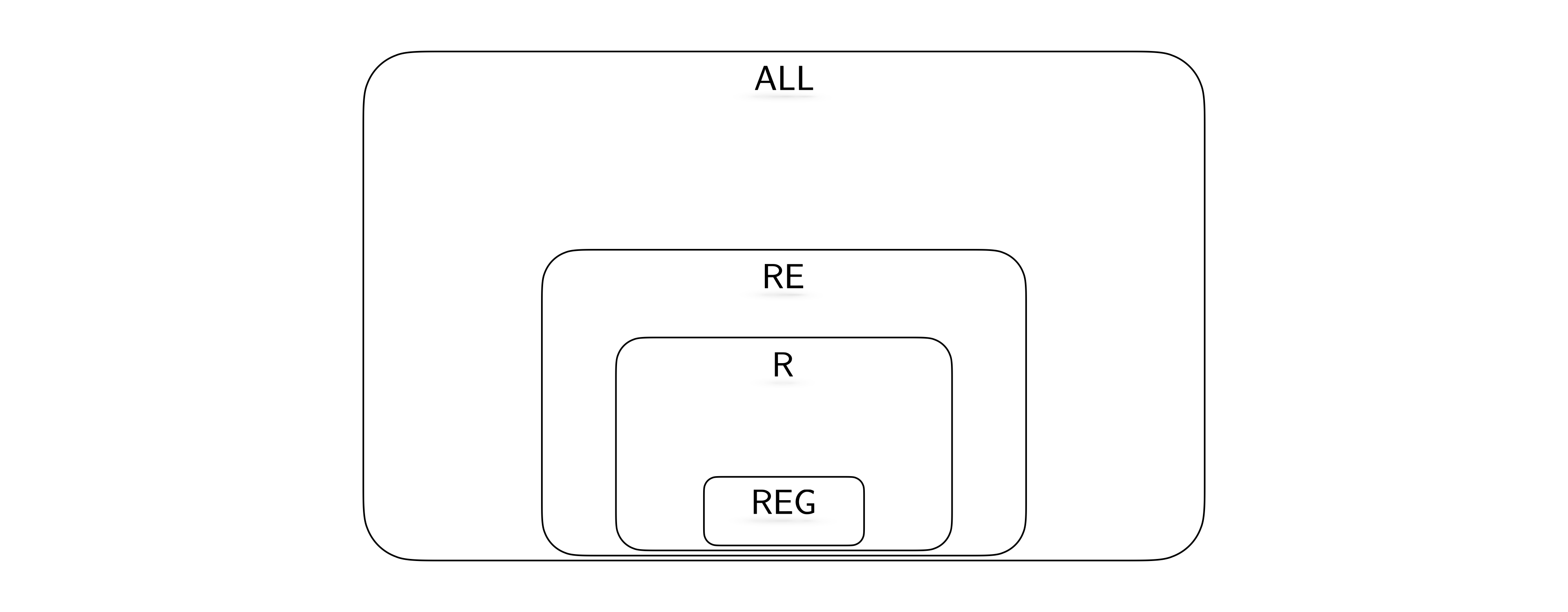
Furthermore, we know $\{{\texttt{0}}^n {\texttt{1}}^n : n \in \mathbb N\}$ is decidable, but not regular. Therefore we know that the first inclusion above is strict. We will next investigate whether the other inclusions are strict or not.

6. Check Your Understanding

Problem

What are the $7$ components in the formal definition of a Turing machine?
True or false: It is possible that in the definition of a TM, $\Sigma = \Gamma$ , where $\Sigma$ is the input alphabet, and $\Gamma$ is the tape alphabet.
True or false: On every valid input, any TM either accepts or rejects.
In the $7$ -tuple definition of a TM, the tape does not appear. Why is this the case?
What is the set of all possible inputs for a TM $M = (Q, \Sigma, \Gamma, \delta, q_0, q_\text{acc}, q_\text{rej})$ ?
In the definition of a TM, the number of states is restricted to be finite. What is the reason for this restriction?
State 4 differences between TMs and DFAs.
True or false: Consider a TM such that the starting state $q_0$ is also the accepting state $q_\text{acc}$ . It is possible that this TM does not halt on some inputs.
Let $D = (Q, \Sigma, \delta, q_0, F)$ be a DFA. Define a decider TM $M$ (specifying the components of the 7-tuple) such that $L(M) = L(D)$ .
What are the 3 components of a configuration of a Turing machine? How is a configuration typically written?
True or false: We say that a language $K$ is a decidable language if there exists a Turing machine $M$ such that $K = L(M)$ .
What is a decider TM?
True or false: For each decidable language, there is exactly one TM that decides it.
What do we mean when we say “a high-level description of a TM”?
What is a universal TM?
True or false: A universal TM is a decider.
What is the Church-Turing thesis?
What is the significance of the Church-Turing thesis?
True or false: $L \subseteq \Sigma^*$ is undecidable if and only if $\Sigma^* \backslash L$ is undecidable.
Is the following statement true, false, or hard to determine with the knowledge we have so far? $\varnothing$ is decidable.
Is the following statement true, false, or hard to determine with the knowledge we have so far? $\Sigma^*$ is decidable.
Is the following statement true, false, or hard to determine with the knowledge we have so far? The language $\{\left \langle M \right\rangle : \text{$M$ is a TM with $L(M) \neq \varnothing$}\}$ is decidable.
True or false: Let $L \subseteq \{{\texttt{0}},{\texttt{1}}\}^*$ be defined as follows: $L = \begin{cases} \{{\texttt{0}}^n{\texttt{1}}^n : n \in \mathbb N\} & \text{if the Goldbach conjecture is true;} \\ \{{\texttt{1}}^{2^n} : n \in \mathbb N\} & \text{otherwise.} \end{cases}$ $L$ is decidable. (Feel free to Google what Goldbach conjecture is.)
Let $L$ and $K$ be two languages. What does “ $L$ reduces to $K$ ” mean? Give an example of $L$ and $K$ such that $L$ reduces to $K$ .

7. High-Order Bits

Important Note

Here are the important things to keep in mind from this chapter.

Understand the key differences and similarities between DFAs and TMs are.
Given a TM, describe in English the language that it solves.
Given the description of a decidable language, come up with a TM that decides it. Note that there are various ways we can describe a TM (what we refer to as the low level, medium level, and the high level representations). You may need to present a TM in any of these levels.
What is the definition of a configuration and why is it important?
The TM computational model describes a very simple programming language.
Even though the definition of a TM is far simpler than any other programming language that you use, convince yourself that it is powerful enough to capture any computation that can be expressed in your favorite programming language. This is a fact that can be proved formally, but we do not do so since it would be extremely long and tedious.
What is the Church-Turing thesis and what does it imply? Note that we do not need to invoke the Church-Turing thesis for the previous point. The Church-Turing thesis is a much stronger claim. It captures our belief that any kind of algorithm that can be carried out by any kind of a natural process can be simulated on a Turing machine. This is not a mathematical statement that can be proved but rather a statement about our universe and the laws of physics.
The set of Turing machines is encodable (i.e. every TM can be represented using a finite-length string). This implies that an algorithm (or Turing machine) can take as input (the encoding of) another Turing machine. This idea is the basis for the universal Turing machine. It allows us to have one (universal) machine/algorithm that can simulate any other machine/algorithm that is given as input.
This chapter contains several algorithms that take encodings of DFAs as input. So these are algorithms that take as input the text representations of other algorithms. There are several interesting questions that one might want to answer given the code of an algorithm (i.e. does it accept a certain input, do two algorithms with different representations solve exactly the same computational problem, etc.) We explore some of these questions in the context of DFAs. It is important you get used to the idea of treating code (which may represent a DFA or a TM) as data/input.
This chapter also introduces the idea of a reduction (the idea of solving a computational problem by using, as a helper function, an algorithm that solves a different problem). Reductions will come up again in future chapters, and it is important that you have a solid understanding of what it means.

Uncountable Sets

1. Comparison of Sets

Definition (Injection, surjection, and bijection)

Let $X$ and $Y$ be two (possibly infinite) sets.

A function $f: X \to Y$ is called injective if for any $x,x' \in X$ such that $x \neq x'$ , we have $f(x) \neq f(x')$ . We write $X \hookrightarrow Y$ if there exists an injective function from $X$ to $Y$ .
A function $f: X \to Y$ is called surjective if for all $y \in Y$ , there exists an $x \in X$ such that $f(x) = y$ . We write $X \twoheadrightarrow Y$ if there exists a surjective function from $X$ to $Y$ .
A function $f: X \to Y$ is called bijective (or one-to-one correspondence) if it is both injective and surjective. We write $X \leftrightarrow Y$ if there exists a bijective function from $X$ to $Y$ .

Theorem (Relationships between different types of functions)

Let $X, Y$ and $Z$ be three (possibly infinite) sets. Then,

$X \hookrightarrow Y$ if and only if $Y \twoheadrightarrow X$ ;
if $X \hookrightarrow Y$ and $Y \hookrightarrow Z$ , then $X \hookrightarrow Z$ ;
$X \leftrightarrow Y$ if and only if $X \hookrightarrow Y$ and $Y \hookrightarrow X$ .

Definition (Comparison of cardinality of sets)

Let $X$ and $Y$ be two sets.

We write $|X| = |Y|$ if $X \leftrightarrow Y$ .
We write $|X| \leq |Y|$ (or $|Y| \geq |X|$ ) if $X \hookrightarrow Y$ , or equivalently, if $Y \twoheadrightarrow X$ .
We write $|X| < |Y|$ (or $|Y| > |X|$ ) if it is not the case that $|X| \geq |Y|$ .

Remark (Sanity checks for comparing cardinality of sets)

Theorem (Relationships between different types of functions) justifies the use of the notation $=$ , $\leq$ , $\geq$ , $<$ and $>$ . The properties we would expect to hold for this type of notation indeed do hold. For example,

$|X| = |Y|$ if and only if $|X| \leq |Y|$ and $|Y| \leq |X|$ ,
if $|X| \leq |Y| \leq |Z|$ , then $|X| \leq |Z|$ ,
if $|X| \leq |Y| < |Z|$ , then $|X| < |Z|$ , and so on.

Note (Set inclusion vs cardinality)

If $X \subseteq Y$ , then $|X| \leq |Y|$ since the identity function that maps $x \in X$ to $x \in Y$ is an injection.

Proposition (

|\mathbb S| = |\mathbb N|

)

Let $\mathbb S= \{0, 1, 4, 9,\ldots\}$ be the set of squares. Then $|\mathbb S| = |\mathbb N|$ .

Proposition (

|\mathbb Z| = |\mathbb N|

)

Let $\mathbb Z$ be the set of integers. Then $|\mathbb Z| = |\mathbb N|$ .

Proposition (

|\mathbb Z\times \mathbb Z| = |\mathbb N|

)

Let $\mathbb Z\times \mathbb Z$ be the set of tuples with integer coordinates. Then $|\mathbb Z\times \mathbb Z| = |\mathbb N|$ .

Proposition (

|\mathbb Q| = |\mathbb N|

)

Let $\mathbb Q$ be the set of rational numbers. Then $|\mathbb Q| = |\mathbb N|$ .

Proposition (

|\Sigma^*| = |\mathbb N|

)

Let $\Sigma$ be a finite non-empty set. Then $|\Sigma^*| = |\mathbb N|$ .

Theorem (No cardinality strictly between finite and

|\mathbb N|

)

If $S$ is an infinite set and $|S| \leq |\mathbb N|$ , then $|S| = |\mathbb N|$ .

Exercise (Proof of no cardinality strictly between finite and

|\mathbb N|

)

Prove the above theorem.

Proposition (

|\mathbb{P}| = |\mathbb N|

)

Let $\mathbb{P} = \{2, 3, 5, 7, \ldots\}$ be the set of prime numbers. Then $|\mathbb{P}| = |\mathbb N|$ .

2. Countable Sets

Definition (Countable and uncountable sets)

A set $S$ is called countable if $|S| \leq |\mathbb N|$ .
A set $S$ is called countably infinite if it is countable and infinite.
A set $S$ is called uncountable if it is not countable, i.e. $|S| > |\mathbb N|$ .

Note (Only two options for countable sets)

Theorem (No cardinality strictly between finite and $|\mathbb N|$ ) implies that if $S$ is countable, there are two options: either $S$ is finite, or $|S| = |\mathbb N|$ .

Important Note (Countability is equivalent to encodability)

Recall that a set $S$ is encodable if for some alphabet $\Sigma$ , there is an injection from $S$ to $\Sigma^*$ , or equivalently, $|S| \leq |\Sigma^*|$ (Definition (Encoding elements of a set)). Since $|\mathbb N| = |\Sigma^*|$ , we see that a set is countable if and only if it is encodable. Therefore, one can show that a set is countable by showing that it is encodable. We will call this the “CS method” for showing countability.

The standard definition of countability ( $|S| \leq |\mathbb N|$ ) highlights the following heuristic.

If you can list the elements of $S$ in a way that every element appears in the list eventually, then $S$ is countable.

The encodability definition highlights another heuristic that is familiar in computer science.

If you can “write down” each element of $S$ using a finite number of symbols, then $S$ is countable.

Proposition (The set of polynomials with rational coefficients is countable)

The set of all polynomials in one variable with rational coefficients is countable.

Exercise (Practice with countability proofs)

Show that the following sets are countable using the CS method.

$\mathbb Z\times \mathbb Z\times \mathbb Z$ .
The set of all functions $f: S \to \mathbb N$ , where $S$ is some fixed finite set.

3. Diagonalization and Uncountable Sets

Note (Functions in disguise)

The following are some examples of how various mathematical objects have a natural representation as a function.

Sets. A set $S \subseteq X$ can be viewed as a function $f_S: X \to \{0,1\}$ , where $f_S(x) = 1$ if and only if $x \in S$ . This is called the characteristic function of the set. Recall that we made this observation in Important Note (Correspondence between decision problems and languages).
Finite sequences. A sequence $s$ of length $k$ with elements from a set $Y$ can be viewed as a function $f_s : \{0,1,2,\ldots,k-1\} \to Y$ , where $f_s(i)$ is the $i$ ’th element of the sequence (starting counting from $0$ ). In other words, given $f_s$ , the corresponding sequence is $(f_s(0), f_s(1), \ldots, f_s(k-1))$ .
Infinite sequences. Similarly, an infinite-length sequence $s$ with elements from $Y$ can be viewed as a function $f_s : \mathbb N\to Y$ .
Numbers. Numbers can be viewed as functions since the binary representation of a number is a sequence of bits (possibly infinite-length).

For example, all real numbers between $0$ and $1$ (inclusive) is denoted by $[0,1]$ . Every function $f : \mathbb N\to \{0,1\}$ represents a real number in $[0,1]$ in binary, namely $0.f(0)f(1)f(2)\ldots$ .

Lemma (Diagonalization)

Let $X$ be any set, and let $\mathcal{F}$ be a set of functions $f: X \to Y$ where $|Y| \geq 2$ . If $|X| \geq |\mathcal{F}|$ , we can construct a function $f_D : X \to Y$ such that $f_D \not \in \mathcal{F}$ .

Remark (There are many choices for the diagonal element)

When we apply the above lemma to construct an explicit $f_D \not\in \mathcal{F}$ , we call that diagonalizing against the set $\mathcal{F}$ . And we call $f_D$ a diagonal element. Typically there are several choices for the definition of $f_D$ :

Different injections $\phi : \mathcal{F}\to X$ can lead to different diagonal elements.
If $|Y| > 2$ , we have more than one choice on what value we assign to $f_D(x_f)$ that makes $f_D(x_f) \neq f(x_f)$ (here $x_f$ denotes $\phi(f)$ ).
If there are elements $x \in X$ not in the range of $\phi$ , then we can define $f_D(x)$ any way we like.

Important Note (Diagonalization gives an explicit construction)

Note that diagonalizing against a set $\mathcal{F}$ produces an explicit function $f_D$ not in $\mathcal{F}$ . Therefore, in situations where you wish to find an explicit object that is not in a given set, you should consider if diagonalization could be applied.

Corollary (Direct corollary of diagonalization)

If $\mathcal{F}$ is the set of all functions $f: X \to Y$ (and $|Y| \geq 2$ ), then $|X| < |\mathcal{F}|$ .

Exercise (Diagonalization and uncountability)

Using the corollary above, give an example of an uncountable set.

Theorem (Cantor’s Theorem)

For any set $X$ , $|X| < |\wp(X)|$ .

Remark (Russell’s Paradox as diagonalization)

In the famous Russell’s Paradox, we consider the set of all sets that do not contain themselves. That is, we consider $D = \{\text{set } S : S \not \in S\}.$ Then we ask whether $D$ is in $D$ or not. If $D \in D$ , then by the definition of $D$ , $D \not \in D$ . And if $D \not \in D$ , again by the definition of $D$ , $D \in D$ . Either way we get a contradiction. Therefore, the conclusion is that such a set $D$ should not be mathematically definable.

This paradox is also an application of diagonalization. For any set $X$ , we cannot diagonalize against the set of all functions $f : X \to \{0,1\}$ . If we imagine diagonalizing against this set, where $X$ is the set of all sets, the natural diagonal element $f_D$ that comes out of diagonalization is precisely the characteristic function of the set $D$ defined above.

Corollary (The power set of an infinite set is uncountable)

For any infinite set $S$ , $\wp(S)$ is uncountable. In particular, $\wp(\mathbb N)$ is uncountable.

Note (Diagonalization with countable sets)

In a common scenario where diagonalization is applied, both $\mathcal{F}$ and $X$ are countably infinite sets. So we can list the elements of $\mathcal{F}$ as $f_1,\; f_2,\; f_3,\; \ldots$ as well as the elements of $X$ as $x_1,\; x_2,\; x_3,\; \ldots$ Then for all $i$ , define $f_D(x_i)$ such that $f_D(x_i) \neq f_i(x_i)$ . If $Y = \{0,1\}$ , for example, $f_D(x_i) = \textbf{not} \; f_i(x_i)$ . The construction of $f_D$ can be nicely visualized with a table, as shown below. Here, an entry corresponding to row $f_i$ and column $x_j$ contains the value $f_i(x_j)$ .

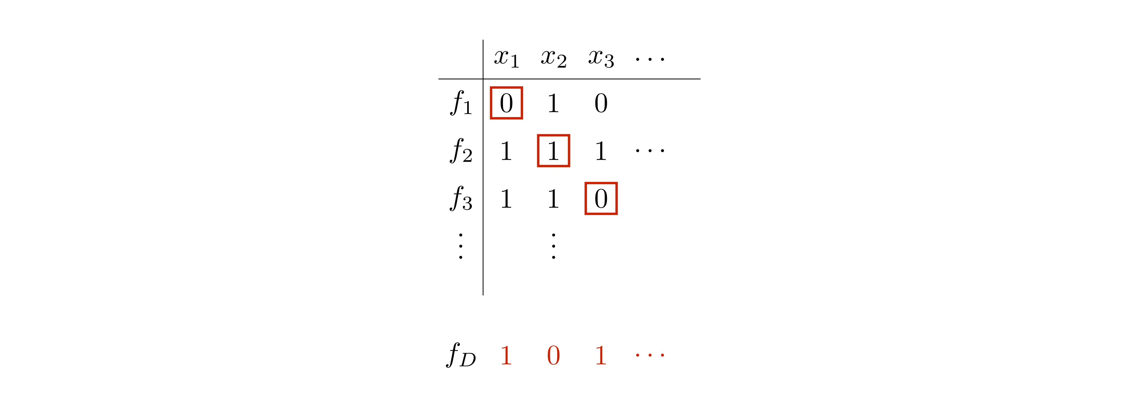
By construction, the diagonal element $f_D$ differs from every $f_i$ , $i \in \{1,2,3,\ldots\}$ . In particular, it differs from $f_i$ with respect to the input $x_i$ .

Proposition (Irrational numbers exist)

There exists an irrational real number, that is, there exists a number in $\mathbb R\setminus \mathbb Q$ .

Exercise (

\mathbb R

is uncountable)

Prove that $\mathbb R$ is uncountable.

Definition (

\Sigma^\infty

)

Let $\Sigma$ be some finite alphabet. We denote by $\Sigma^\infty$ the set of all infinite length words over the alphabet $\Sigma$ .

Theorem (

\{{\texttt{0}},{\texttt{1}}\}^\infty

is uncountable)

The set $\{{\texttt{0}},{\texttt{1}}\}^\infty$ is uncountable.

Exercise (Uncountable sets are closed under supersets)

Prove that if $X$ is uncountable and $X \subseteq Y$ , then $Y$ is also uncountable.

Important Note (Uncountability via

\{{\texttt{0}},{\texttt{1}}\}^\infty

)

If we want to show that a set $X$ is uncountable, it suffices to show that $|X| \geq |Y|$ for some uncountable set $Y$ . Typically, a good choice for such a $Y$ is $\{{\texttt{0}},{\texttt{1}}\}^\infty$ . And one strategy for establishing $|X| \geq |\{{\texttt{0}},{\texttt{1}}\}^\infty|$ is to identify a subset $S$ of $X$ such that $S \leftrightarrow\{{\texttt{0}},{\texttt{1}}\}^\infty$ .

Exercise (Practice with uncountability proofs)

Show that the following sets are uncountable.

The set of all bijective functions from $\mathbb N$ to $\mathbb N$ .
$\{x_1x_2 x_3 \ldots \in \{{\texttt{1}},{\texttt{2}}\}^\infty : \text{ for all $n \geq 1$, $\; \sum_{i=1}^n x_i \not\equiv 0 \mod 4$}\}$

4. Check Your Understanding

Problem

For sets $X, Y$ , what are the definitions of $|X| \leq |Y|$ , $|X| \geq |Y|$ , $|X| = |Y|$ , and $|X| < |Y|$ ?
What is the definition of a countable set?
What is the CS method for showing that a set is countable?
True or false: There exists an infinite set $S$ such that $|S| < |\mathbb N|$ .
True or false: $\{{\texttt{0}},{\texttt{1}}\}^* \cap \{{\texttt{0}},{\texttt{1}}\}^\infty = \varnothing$ .
True or false: $|\{{\texttt{0}},{\texttt{1}},{\texttt{2}}\}^*| = |\mathbb Q\times \mathbb Q|$ .
State the Diagonalization Lemma and specify how the diagonal function $f_D : X \to Y$ is constructed (the construction should make sense for any $X$ so do not assume $X$ is finite or countably infinite).
What is the connection between Diagonalization Lemma and uncountability?
What is Cantor’s Theorem?
True or false: $|\wp(\{{\texttt{0}},{\texttt{1}}\}^\infty)| = |\wp(\wp(\{{\texttt{0}},{\texttt{1}}\}^\infty))|$ .
True or false: There is a surjection from $\{{\texttt{0}},{\texttt{1}}\}^\infty$ to $\{{\texttt{0}},{\texttt{1}},{\texttt{2}},{\texttt{3}}\}^\infty$ .
True or false: Let $\Sigma$ be an alphabet. The set of encodings mapping $\mathbb N$ to $\Sigma^*$ is countable.
True or false: Let $\Sigma = \{{\texttt{1}}\}$ be a unary alphabet. The set of all languages over $\Sigma$ is countable.
State a technique for proving that a given set is uncountable.

5. High-Order Bits

Important Note

Here are the important things to keep in mind from this chapter.

The definitions of injective, surjective and bijective functions are fundamental.
The concepts of countable and uncountable sets, and their precise mathematical definitions.
When it comes to showing that a set is countable, the CS method is the best choice, almost always.
The Diagonalization Lemma is one of the most important and powerful techniques in all mathematics.
When showing that a set is uncountable, establishing an injection from $\{0,1\}^\infty$ (or a surjection to $\{{\texttt{0}},{\texttt{1}}\}^\infty$ ) is one of the best techniques you can use.

Undecidable Languages

1. Existence of Undecidable Languages

Proposition (The set of Turing machines is countable)

Fix some input alphabet and tape alphabet. The set of all Turing machines $\mathcal{T}= \{M : M \text{ is a TM}\}$ is countable.

Theorem (Almost all languages are undecidable)

Fix some alphabet $\Sigma$ . There are languages $L \subseteq \Sigma^*$ that are not semi-decidable (and therefore undecidable as well).

2. An Explicit Undecidable Language

Note (Diagonalization against a set of function-like objects)

In the previous chapter, we presented diagonalization with respect to a set of functions. However, Lemma (Diagonalization) can be applied in a slightly more general setting: it can be applied when $\mathcal{F}$ is a set of objects that map elements of $X$ to elements of $Y$ (e.g. $\mathcal{F}$ can be a set of Turing machines which map elements of $\Sigma^*$ to elements of $\{0,1,\infty\}$ ). In other words, elements of $\mathcal{F}$ do not have to be functions as long as they are “function-like”. Once diagonalization is applied, one gets an explicit function $f_D : X \to Y$ such that no object in $\mathcal{F}$ matches the input/output behavior of $f_D$ . We will illustrate this in the proof of the next theorem.

Definition (The

\text{SELF-ACCEPTS}_{\text{TM}}

language/problem)

We say that a TM $M$ self-accepts if $M(\left \langle M \right\rangle) = 1$ . The self-accepts problem is defined as the decision problem corresponding to the language $\text{SA}_{\text{TM}}= \text{SELF-ACCEPTS}_{\text{TM}}= \{\left \langle M \right\rangle : \text{$M$ is a TM which self-accepts} \}.$ The complement problem corresponds to the language $\overline{\text{SA}_{\text{TM}}}= \overline{\text{SELF-ACCEPTS}_{\text{TM}}}= \{\left \langle M \right\rangle : \text{$M$ is a TM which does not self-accept}\}.$ Note that if a TM $M$ does not self-accept, then $M(\left \langle M \right\rangle) \in \{0, \infty\}$ .

Theorem (Turing’s 1st Undecidability Theorem)

The language $\overline{\text{SA}_{\text{TM}}}$ is undecidable.

Note (

\overline{\text{SA}_{\text{TM}}}

is not semi-decidable)

Note that the proof of the above theorem establishes something stronger: the language $\overline{\text{SA}_{\text{TM}}}$ is not semi-decidable. To see this, recall that if $M$ is a semi-decider for $f_D$ , by definition, this implies that for all $x \in \Sigma^*$ :

if $f_D(x) = 1$ , then $M(x) = 1$ ,
if $f_D(x) = 0$ , then $M(x) \in \{0, \infty\}$ .

However, by construction of $f_D$ , we know that for input $x = \left \langle M \right\rangle$ , if $f_D(\left \langle M \right\rangle) = 1$ then $M(\left \langle M \right\rangle) \in \{0, \infty\}$ , and if $f_D(\left \langle M \right\rangle) = 0$ , then $M(\left \langle M \right\rangle) = 1$ . So for all TMs $M$ , $M$ fails to semi-decide $f_D$ on input $x = \left \langle M \right\rangle$ .

3. More Undecidable Languages

Theorem (

\text{SA}_{\text{TM}}

is undecidable)

The language $\text{SA}_{\text{TM}}$ is undecidable.

Note (The complement of an undecidable language is undecidable)

The general principle that the above theorem highlights is that since decidable languages are closed under complementation, if $L$ is an undecidable language, then $\overline{L} = \Sigma^* \setminus L$ must also be undecidable.

Definition (

\text{ACCEPTS}

and

\text{HALTS}

for TMs)

We define the following languages: $\begin{aligned} \text{ACCEPTS}_{\text{TM}}& = \{\left \langle M,x \right\rangle : \text{$M$ is a TM which accepts input $x$}\}, \\ \text{HALTS}_{\text{TM}}& = \{\left \langle M,x \right\rangle : \text{$M$ is a TM which halts on input $x$} \}, \\ \end{aligned}$

Theorem (

\text{ACCEPTS}_{\text{TM}}

is undecidable)

The language $\text{ACCEPTS}_{\text{TM}}$ is undecidable.

Theorem (

\text{HALTS}_{\text{TM}}

is undecidable)

The language $\text{HALTS}_{\text{TM}}$ is undecidable.

Proposition (

\text{SA}_{\text{TM}}

\text{ACCEPTS}_{\text{TM}}

\text{HALTS}_{\text{TM}}

are semi-decidable)

The languages $\text{SA}_{\text{TM}}$ , $\text{ACCEPTS}_{\text{TM}}$ , and $\text{HALTS}_{\text{TM}}$ are all semi-decidable, i.e., they are all in $\mathsf{RE}$ .

Theorem (

\mathsf{R}\neq \mathsf{RE}

)

$\mathsf{R}\neq \mathsf{RE}$ .

4. Undecidability Proofs by Reductions

Important Note (Undecidability proofs by reduction)

In the last section, we have used the same technique in all the proofs. It will be convenient to abstract away this technique and give it a name. Fix some alphabet $\Sigma$ . Let $L$ and $K$ be two languages. We say that $L$ reduces to $K$ , written $L \leq K$ , if we are able to do the following: assume $K$ is decidable (for the sake of argument), and then show that $L$ is decidable by using the decider for $K$ as a black-box subroutine (i.e. a helper function). Here the languages $L$ and $K$ may or may not be decidable to begin with. But observe that if $L \leq K$ and $K$ is decidable, then $L$ is also decidable. Or in other words, if $L \leq K$ and $K \in \mathsf{R}$ , then $L \in \mathsf{R}$ . Equivalently, taking the contrapositive, if $L \leq K$ and $L$ is undecidable, then $K$ is also undecidable. So when $L \leq K$ , we think of $K$ as being at least as hard as $L$ with respect to decidability (or that $L$ is no harder than $K$ ), which justifies using the less-than-or-equal-to sign.

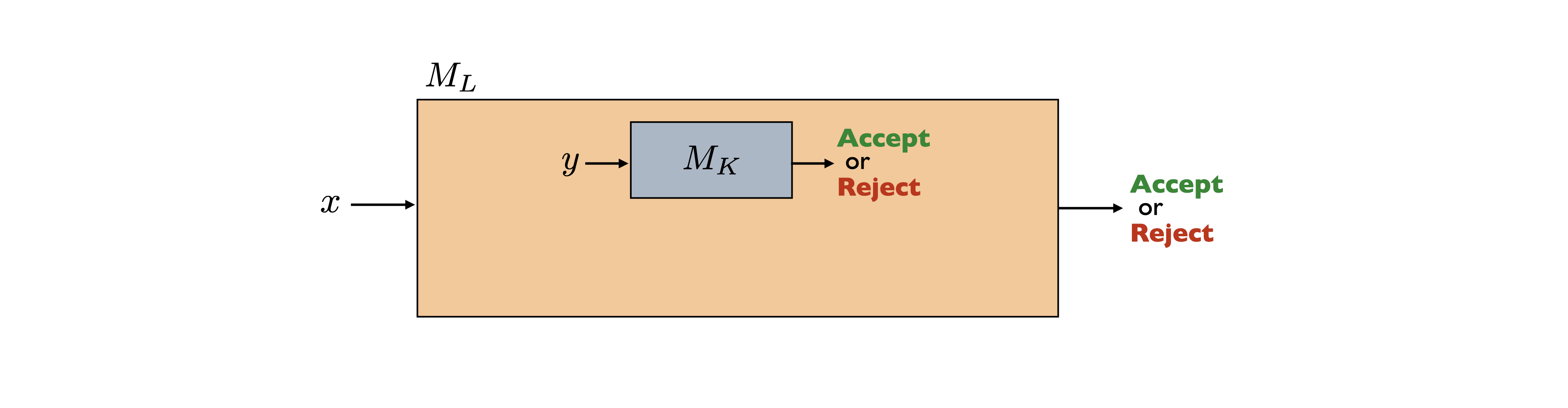
Even though in the diagram above we have drawn one instance of $M_K$ being called within $M_L$ , $M_L$ is allowed to call $M_K$ multiple times with different inputs.

Remark (Turing reductions)

In the literature, the above idea is formalized using the notion of a Turing reduction (with the corresponding symbol $\leq_T$ ). In order to define it formally, we need to define Turing machines that have access to an oracle. See Section (Bonus: Oracle Turing Machines) for details.

Remark (Reductions vs comparing cardinalities)

Note the difference between the notations $|L| \leq |K|$ and $L \leq K$ . These have very different meanings. The notation $L \leq K$ only applies to languages and denotes a reduction. The notation $|L| \leq |K|$ applies to any two sets $L$ and $K$ and denotes the existence of an injective function from the set $L$ to the set $K$ .

Note (Mapping reductions)

Many reductions $L \leq K$ have the following very special structure. The TM $M_L$ is such that on input $x$ , it first transforms $x$ into a new string $y = f(x)$ by applying some computable transformation $f$ . Then $f(x)$ is fed into $M_K$ . The output of $M_L$ is the same as the output of $M_K$ . In other words $M_L(x) = M_K(f(x))$ .

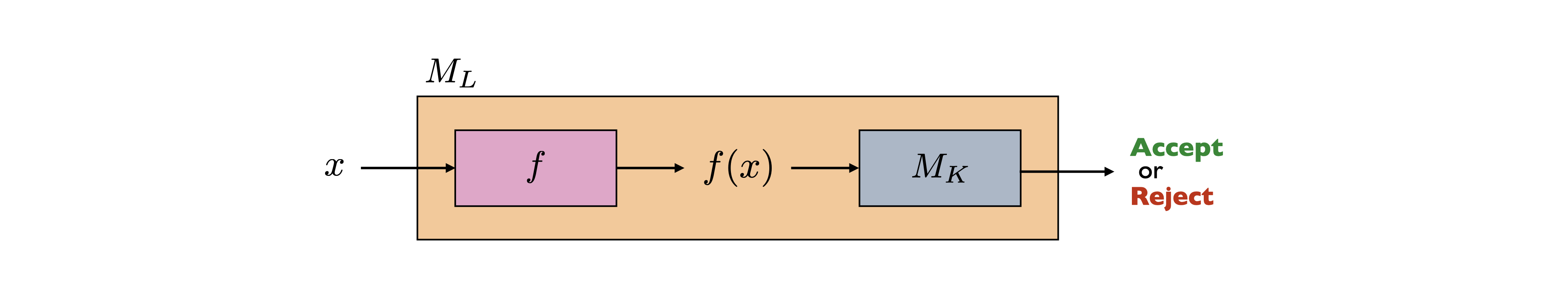
These special kinds of reductions are called mapping reductions (or many-one reductions), with the corresponding notation $L \leq_m K$ . Note that the reduction we have seen from $\text{SA}_{\text{TM}}$ to $\text{ACCEPTS}_{\text{TM}}$ is a mapping reduction. However, the reduction from $\overline{\text{SA}_{\text{TM}}}$ to $\text{SA}_{\text{TM}}$ is not a mapping reduction because the output of $M_K$ is flipped, or in other words, we have $M_L(x) = \textbf{not } M_K(f(x))$ .

Almost all the reductions in this section will be mapping reductions.

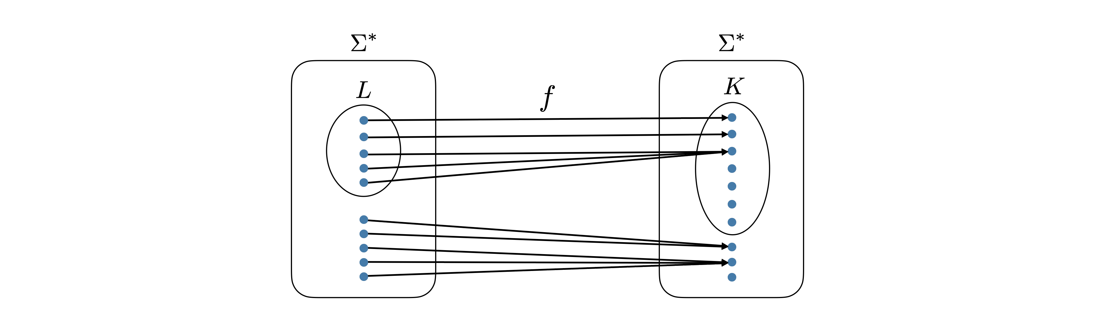
Note that to specify a mapping reduction from $L$ to $K$ , all one needs to do is specify a TM $M_f$ that computes $f : \Sigma^* \to \Sigma^*$ with the property that for any $x \in \Sigma^*$ , $x \in L$ if and only if $f(x) \in K$ .

Definition (More languages related to encodings of TMs)

A TM $M$ is satisfiable if there is some input string that $M$ accepts. In other words, $M$ is satisfiable if $L(M) \neq \varnothing$ . We now define the following languages: $\begin{aligned} \text{SAT}_{\text{TM}}& = \{\left \langle M \right\rangle : \text{$M$ is a satisfiable TM}\}, \\ \text{NEQ}_{\text{TM}}& = \{\left \langle M_1,M_2 \right\rangle : \text{$M_1$ and $M_2$ are TMs with $L(M_1) \neq L(M_2)$}\}, \\ \text{HALTS-EMPTY}_{\text{TM}}& = \{\left \langle M \right\rangle : \text{$M$ is a TM such that $M(\epsilon)$ halts}\}, \\ \text{FINITE}_{\text{TM}}& = \{\left \langle M \right\rangle : \text{$M$ is a TM such that $L(M)$ is finite}\}.\end{aligned}$

Theorem (

\text{SAT}_{\text{TM}}

is undecidable)

The language $\text{SAT}_{\text{TM}}$ is undecidable.

Theorem (

\text{NEQ}_{\text{TM}}

is undecidable)

The language $\text{NEQ}_{\text{TM}}$ is undecidable.

Exercise (Practice with undecidability proofs)

Show that the following languages are undecidable.

$\text{HALTS-EMPTY}_{\text{TM}}= \{\left \langle M \right\rangle : \text{ $M$ is a TM and $M(\epsilon)$ halts}\}$
$\text{FINITE}_{\text{TM}}= \{\left \langle M \right\rangle : \text{$M$ is a TM that accepts finitely many strings}\}$

Theorem (

\text{SAT}_{\text{TM}}\leq \text{HALTS}_{\text{TM}}

)

$\text{SAT}_{\text{TM}}\leq \text{HALTS}_{\text{TM}}$ .

Exercise (

\text{SAT}_{\text{TM}}

is in

\mathsf{RE}

)

Describe a TM that semi-decides $\text{SAT}_{\text{TM}}$ . Proof of correctness is not required.

Exercise (Practice with reduction definition)

Let $L, K \subseteq \{{\texttt{0}},{\texttt{1}}\}^*$ be languages. Prove or disprove the following claims.

If $L \leq K$ then $K \leq L$ .
If $L \leq K$ and $K$ is regular, then $L$ is regular.

Exercise (Calling the helper function more than once)

In all the reductions $L \leq K$ presented in this chapter, the TM $M_L$ calls the TM $M_K$ exactly once. (And in fact, almost all the reductions in this chapter are mapping reductions). Present a reduction from $\text{HALTS}_{\text{TM}}$ to $\text{ACCEPTS}_{\text{TM}}$ in which $M_\text{HALTS}$ calls $M_\text{ACCEPTS}$ twice, and both calls/outputs are used in a meaningful way.

5. Non-Semi-Decidable Languages

Theorem (Non-semi-decidability through semi-decidable undecidable languages)

If a language $L$ is semi-decidable but undecidable, then $\overline{L}$ is not semi-decidable. In other words, if $L \in \mathsf{RE}\setminus \mathsf{R}$ , then $\overline{L} \not \in \mathsf{RE}$ .

Corollary (Non-semi-decidable languages)

The languages $\overline{\text{SA}_{\text{TM}}}$ , $\overline{\text{ACCEPTS}_{\text{TM}}}$ , and $\overline{\text{HALTS}_{\text{TM}}}$ are not semi-decidable, i.e. they are not in $\mathsf{RE}$ .

Note (Comparing

\mathsf{REG}

\mathsf{R}

, and

\mathsf{RE}

)

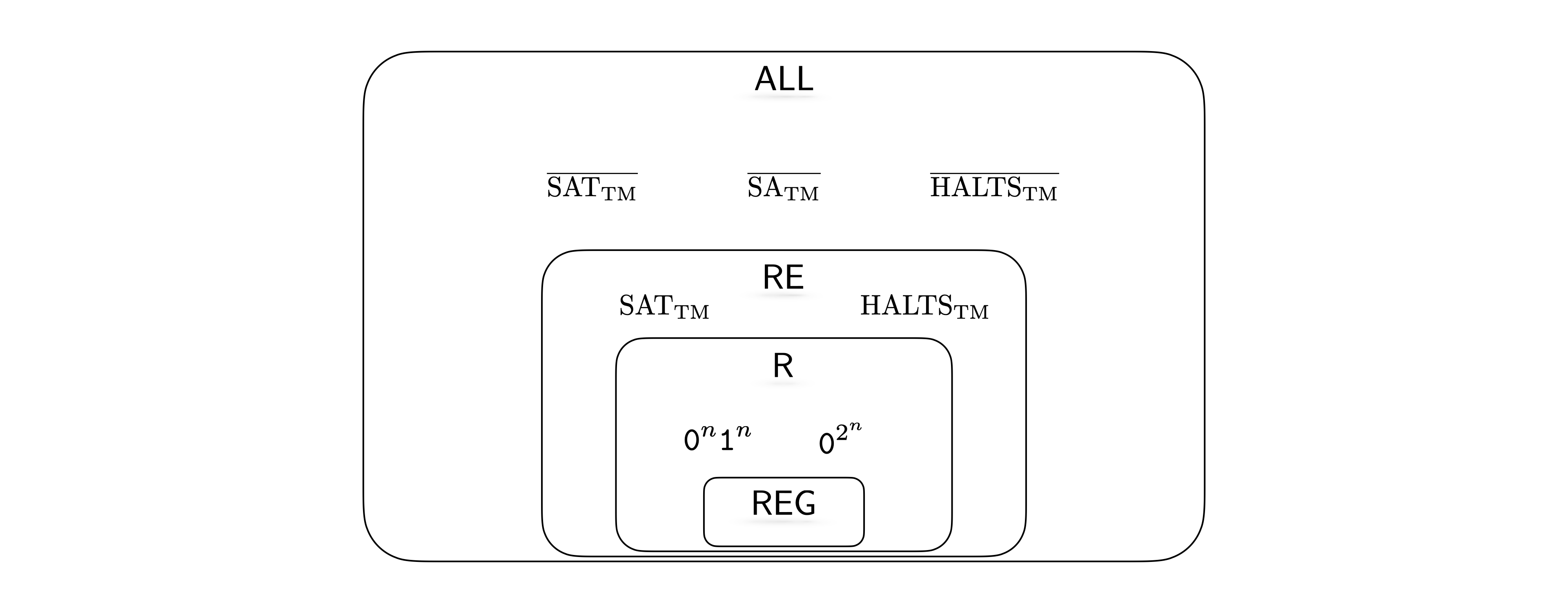
The relationship among the complexity classes $\mathsf{REG}$ , $\mathsf{R}$ , and $\mathsf{RE}$ and can be summarized as follows.

$\mathsf{REG}\subsetneq \mathsf{R}$ since $\{{\texttt{0}}^n{\texttt{1}}^n : n \in \mathbb N\}$ is not regular but is decidable.
There are languages like $\text{SA}_{\text{TM}}$ , $\text{ACCEPTS}_{\text{TM}}$ , $\text{HALTS}_{\text{TM}}$ , $\text{SAT}_{\text{TM}}$ that are undecidable (not in $\mathsf{R}$ ), but are semi-decidable (in $\mathsf{RE}$ ).
The complements of the languages above are not in $\mathsf{RE}$ .

6. Bonus: Oracle Turing Machines

Definition (Oracle Turing machines)

Given some decision problem $g : \Sigma^* \to \{0,1\}$ , we define a $g$ -oracle Turing machine (or simply $g$ -OTM, or just OTM if $g$ is understood from the context) as a Turing machine with an additional oracle instruction which can be used in the TM’s high-level description. The additional instruction has the following form. For any string $x$ and any variable name $y$ of our choosing, we are allowed to use $y = g(x).$ After this instruction, the variable $y$ holds the value $g(x)$ and can be used in the rest of the Turing machine’s description. In this context, the function $g$ is called an oracle.

We’ll use a superscript of $g$ (e.g. $M^g$ ) to indicate that a machine is a $g$ -OTM.

Similar to TMs, we write $M^g(x) = 1$ if the oracle TM $M^g$ , on input $x$ , accepts. We write $M^g(x) = 0$ if it rejects. And we write $M^g(x) = \infty$ if it loops forever.

If $f : \Sigma^* \to \{0,1\}$ is a decision problem such that for all $x \in \Sigma^*$ , $M^g(x) = f(x)$ , then we say $M^g$ describes $f$ (and the language corresponding to $f$ ).

Definition (Turing reduction)

Let $L$ and $K$ be two languages, and let $k$ be the decision problem corresponding to $K$ . We say that $L$ Turing-reduces to $K$ , written $L \leq_T K$ , if there is an oracle Turing machine $M^k$ describing $L$ .

Note (Turing reductions and decidability)

Observe that if $L \leq_T K$ and $K$ is decidable, then $L$ is decidable. This is because if $L \leq_T K$ , then by definition, there is an oracle Turing machine $M^k$ that describes $L$ . If $K$ is decidable, there is a TM $M_K$ deciding $K$ . Then in $M^k$ , if we replace all calls to the oracle $k$ with $M_K$ , we end up with a TM deciding $L$ .

It follows (taking the contrapositive of the observation) that if $L \leq_T K$ and $L$ is undecidable, then $K$ is undecidable.

Important Note (TMs as a description model)

As we have already seen, the set of all languages, $\wp(\Sigma^*)$ , is not encodable. Most languages do not have a finite description. In addition to thinking about the TM model as a computational model, it is useful to also think of it as a finite description model: Every TM finitely describes/defines the language that it decides (or semi-decides).

The TM model is not a comprehensive finite description model. There are many finitely describable languages (e.g., $\overline{\text{SA}_{\text{TM}}}$ , $\text{ACCEPTS}_{\text{TM}}$ , $\text{HALTS}_{\text{TM}}$ ) that a TM cannot finitely describe. The oracle TM model extends the reach of the TM model as a finite description model.

If we inspect the proof of Turing’s 1st Undecidability Theorem, we can see that we never really made use of the fact that TMs represent a computational model. The crucial part of the argument was that the set of TMs is encodable/countable. Or in other words, we only needed that the TM model is a finite description model for languages/decision problems. This means that for other finite description models, like the oracle TM model, we can carry out the same argument.

An important lesson here is that the main limitation Turing’s 1st Undecidability Theorem highlights about TMs is not that they form a computing model, but that they form a finite description model.

Note (Languages involving encodings of oracle TMs)

Fix an oracle $g$ . Then we can define the languages $\text{ACCEPTS}_{\text{OTM}}$ , $\text{HALTS}_{\text{OTM}}$ , $\text{SA}_{\text{OTM}}$ , and so on, analogous to how they are defined for TMs. For example, $\text{HALTS}_{\text{OTM}}= \{\left \langle M^g,x \right\rangle : \text{$M^g$ is a $g$-OTM which halts on input $x$} \}.$

Theorem (Limits of oracle Turing machines)

Fix an oracle $g$ . Then there is no oracle Turing machine that describes $\overline{\text{SA}_{\text{OTM}}}$ .

7. Check Your Understanding

Problem

State 4 languages that are undecidable.
State an undecidable language whose description does not involve Turing machines.
Describe 3 languages that are not semi-decidable.
Describe how one can show that a language is undecidable using the notion of a reduction.
True or false: For languages $K$ and $L$ , if $K \leq L$ , then $L$ is undecidable.
True or false: For languages $K$ and $L$ , if $K \leq L$ and $L \leq K$ , then $L$ and $K$ are both decidable.
True or false: Fix some alphabet $\Sigma$ . The set of regular languages over $\Sigma$ is countable.
True or false: Fix an alphabet $\Sigma$ . The set of undecidable languages is countable.
True or false: Fix an alphabet $\Sigma$ . The set of decidable languages is infinite.
True or false: If languages $K$ and $L$ are both undecidable, then their union is also undecidable.
True or false: If a language $L$ is undecidable, then $L$ is infinite.
True or false: $\Sigma^* \leq \varnothing$ .
True or false: $\text{HALTS}_{\text{TM}}\leq \Sigma^*$ .
True or false: Every decidable language reduces to $\text{HALTS}_{\text{TM}}$ .
True or false: For all unary languages $L$ (i.e. languages over the alphabet $\Sigma = \{{\texttt{1}}\}$ ), $L$ is decidable.
In a previous chapter, we saw that the language $\text{SAT}_{\text{DFA}}$ is decidable. In particular, we saw that given the encoding of a DFA $D$ , we can determine if $D$ accepts a string by checking if in the state diagram of $D$ , there is a directed path from the initial state to one of the accepting states.

In this chapter, we saw that the language $\text{SAT}_{\text{TM}}$ is undecidable. Show that the strategy above that we used for DFAs does not apply to TMs by drawing the state diagram of a TM $M$ with $L(M) = \varnothing$ , but there is a path from the starting state to the accepting state.

8. High-Order Bits

Important Note

Here are the important things to keep in mind from this chapter.

The existence of undecidable languages follows by a counting argument: The set of all languages is uncountable whereas the set of decidable languages is countable. This shows that almost all languages are undecidable, however, it does not give us an explicit undecidable language.
We can use diagonalization to come up with an explicit language that is undecidable.
Reductions are very important. We have seen in an earlier chapter that reductions can be used to expand the landscape of decidable languages. In this chapter, you see that it can be used to expand the landscape of undecidable languages.
This chapter has many examples of undecidability proofs. It is easy to fall in the trap of trying to memorize the template of such proofs rather than really understanding the logic behind how and why these proofs work. If you struggle to understand these proofs, it is usually a sign that there are gaps in your knowledge from previous chapters. Come talk to us so we can help you identify those gaps.

Unprovable Truths

1. Hilbert’s Program

Important Note (Mathematical reasoning is computation)

Note that both $\text{Prover}$ and $\text{Verifier}$ above represent computational processes. So a key part in formalizing $\text{GORM}$ is the formalization of computation. Luckily, we already have a great model for computation: Turing machines.

Note (Formalizing a subarea of mathematical reasoning)

Even though our main interest is formalizing all mathematical reasoning, it is useful to build a general framework for formalizing any subset of mathematical reasoning. For instance, we may want to come up with a formalization that captures mathematical reasoning for plane geometry. Or we may want to formalize basic arithmetic. Or we may want to formalize probability theory. For any area $A$ of mathematical reasoning, we will let $\text{GORM}_A$ denote Good Old Regular Mathematics restricted to $A$ . Without the subscript, $\text{GORM}$ represents all mathematical reasoning.

Proof System

Let $A$ be some area of mathematics. A proof system $\text{PS}_A$ for $A$ is a mathematical formalization of $\text{GORM}_A$ with the following properties.

For every statement $S$ in $\text{GORM}_A$ with a truth value, there is a precise representation of $S$ in $\text{PS}_A$ .
For every argument $P$ in $\text{GORM}_A$ , there is a precise representation of $P$ in $\text{PS}_A$ .
$\text{PS}_A$ specifies a decider TM $V$ (called a verifier) such that $V(\left \langle S,P \right\rangle)$ accepts if and only if $P$ is a proof of $S$ .

Since the verification process represents a computation, there is an implicit requirement that the set of statements in $\text{PS}_A$ as well as the set of proofs in $\text{PS}_A$ are encodable.

Definition (Provable, refutable, resolvable, independent)

Let $\text{PS}$ be a proof system and let $S$ be a statement in $\text{PS}$ .

Statement $S$ is provable means there is a proof of $S$ in $\text{PS}$ .
- If $S$ is provable, we say $\text{PS}$ proves $S$ .
- We use $\text{Provable}(\cdot)$ to denote the function such that $\text{Provable}(\left \langle S \right\rangle)$ returns True if and only if $S$ is provable. We can view $\text{Provable}(\cdot)$ as a decision problem.
Statement $S$ is refutable means $\text{PS}$ proves the negation of $S$ , (i.e. ${\neg S}$ ).
Statement $S$ is resolvable means that $S$ is either provable or refutable.
If statement $S$ is not resolvable, we say $S$ is independent of $\text{PS}$ .

Definition (Consistent, sound, complete, decidable)

Let $\text{PS}$ be a proof system.

$\text{PS}$ is consistent means for all $S$ , if $S$ is provable, then ${\neg S}$ is not provable. Or equivalently, for all $S$ , at most one of $S$ and ${\neg S}$ is provable.
$\text{PS}$ is sound means for all $S$ , if $S$ is provable, then $S$ is true (i.e. $\text{Provable}(\left \langle S \right\rangle) \to S$ ). This is equivalent to saying $\text{PS}$ does not prove false statements.
$\text{PS}$ is complete means every statement in $\text{PS}$ is resolvable. Or equivalently, for all $S$ , at least one of $S$ and ${\neg S}$ is provable.
$\text{PS}$ is decidable means that the $\text{Provable}$ decision problem is decidable.

Note (Observations about properties of proof systems)

If $\text{PS}$ is not consistent, then every statement is provable. To see this, suppose $S$ is such that both $S$ and $\neg S$ are provable. And suppose you want to prove some statement $T$ . Then assume, for the sake of contradiction, $\neg T$ . Then derive $S$ as well as $\neg S$ (both are provable). This is the desired contradiction.
If $\text{PS}$ is sound, then it must be consistent. So we think of soundness as a stronger requirement.
If $\text{PS}$ is both consistent and complete, then for all statements $S$ , exactly one of $S$ and ${\neg S}$ is provable.
If $\text{PS}$ is both sound and complete, then in addition to the observation in the previous point, provable statements would be true. So for all statements $S$ , we would have $S \leftrightarrow\text{Provable}(\left \langle S \right\rangle)$ , and truth would correspond exactly to provability.
It is not hard to see that for any proof system $\text{PS}$ , $\text{Provable}$ is semi-decidable. Recalling Definition (TM semi-deciding a language or decision problem), to show that $\text{Provable}$ is semi-decidable, we need to come up with a TM $M$ such that if $S$ is provable, $M(\left \langle S \right\rangle)$ accepts, and if $S$ is not provable, then $M(\left \langle S \right\rangle)$ does not accept (i.e. rejects or loops forever). The brute-force search algorithm described below accomplishes this. (Recall $V$ denotes the verifier for $\text{PS}$ .) $\begin{aligned} \hline\hline\\[-12pt] &\textbf{def}\;\; M_\text{RESOLVE}(\left \langle S \right\rangle):\\ &{\scriptstyle 1.}~~~~\texttt{For $k = 1, 2, 3, \ldots$}\\ &{\scriptstyle 2.}~~~~~~~~\texttt{For every string $w$ of length $k$:}\\ &{\scriptstyle 3.}~~~~~~~~~~~~\texttt{If $V(\left \langle S, w \right\rangle)$ accepts: return True.}\\ &{\scriptstyle 4.}~~~~~~~~~~~~\texttt{If $V(\left \langle {\neg S}, w \right\rangle)$ accepts: return False.}\\ \hline\hline \end{aligned}$ Note that this is not a decider for $\text{Provable}$ because it is possible that $S$ is not resolvable (i.e. independent), and in that case, $M_\text{RESOLVE}(\left \langle S \right\rangle)$ would loop forever.

Hilbert’s Program

Come up with a proof system $\text{PS}$ that formalizes $\text{GORM}$ , and furthermore:

Prove that $\text{PS}$ is consistent.
Prove that $\text{PS}$ is complete.
Prove that $\text{PS}$ is decidable.

Remark (Proving soundness?)

Here is a fun question to think about. In Hilbert’s program, why doesn’t Hilbert ask for a proof of soundness and instead asks for a proof of consistency?

2. The ZFC Axiomatic System

Note (Gödel’s Completeness Theorem)

It is worth noting that the set of deduction rules that the Hilbert system specifies is known to be complete (this is Gödel’s Completeness Theorem) in the sense that if you are not able to deduce some truth in the Hilbert System, it is not because you did not have enough deduction rules. It must be because you did not have enough axioms (i.e. some truths were not a logical consequence of the axioms).

Important Note (

\text{GORM}

-to-ZFC Thesis)

Every precise mathematical statement and proof that can be expressed in $\text{GORM}$ can be expressed using the ZFC axiomatic proof system. In other words, every $\text{GORM}$ -statement and $\text{GORM}$ -proof has a corresponding ZFC-statement and ZFC-proof.

Note that the Church-Turing Thesis is really a $\text{GORA}$ -to-TM thesis, where $\text{GORA}$ means Good Old Regular Algorithms. It says that any algorithm can be expressed using a TM. Or in other words, every algorithm “compiles down” to a TM.

You should think of $\text{GORM}$ -to-ZFC Thesis in the same light. Every mathematics proof compiles down to a proof in ZFC.

When we are proving properties of algorithms, we don’t really directly work with TMs, but rather appeal to the Church-Turing Thesis: we work with high-level algorithms with the understanding that they can be translated to TMs. Similarly, when we prove properties of mathematical reasoning, we won’t directly work with ZFC, but appeal to the $\text{GORM}$ -to-ZFC Thesis: we will use high-level mathematical statements and proofs with the understanding that they can be translated into ZFC statements and proofs.

3. Gödel’s Incompleteness Theorems

Theorem (Gödel’s 1st Incompleteness Theorem (Soundness version 1))

ZFC cannot be both sound and complete. In other words, if ZFC is sound, then it must be incomplete.

Theorem (Gödel’s 1st Incompleteness Theorem (Soundness version 2))

If ZFC is sound, then the statement $S_{M_D}$ is independent of ZFC.

Lemma (Halting statements are provable)

If $M$ is a TM such that $M(x)$ accepts, then the statement $\text{``}M(x) \text{ accepts}\text{''}$ is provable. Similarly, if $M(x)$ rejects, then the statement $\text{``}M(x) \text{ rejects}\text{''}$ is provable.

Corollary (ZFC plays nice with halting TMs)

Let $M$ be a TM such that $M(x)$ halts. And let $S = \text{``}M(x) \text{ accepts}\text{''}$ . Then if ZFC is consistent, $S \leftrightarrow M_\text{RESOLVE}(\left \langle S \right\rangle)$ (i.e. ZFC is sound with respect to $S$ ).

Theorem (Gödel’s 1st Incompleteness Theorem)

If ZFC is consistent, then the statement $S_{M_D}$ is independent of ZFC.

Corollary

If ZFC is consistent, then $S_{M_D}$ is false.

Definition (Reduction for provability)

We say proving $S$ reduces to proving $T$ (or simply $S$ reduces to $T$ ) if $T \to S$ is provable.

Theorem (Gödel’s 2nd Incompleteness Theorem)

If ZFC is consistent, then the statement “ZFC is consistent” is not provable in ZFC.

Theorem (Continuum hypothesis is independent)

If ZFC is consistent, the Continuum Hypothesis is independent of ZFC.

4. Turing’s 2nd Undecidability Theorem

Theorem (Turing’s 2nd Undecidability Theorem)

If ZFC is sound, then $\text{Provable}$ is undecidable.

Time Complexity

1. Big-O, Big-Omega and Theta

Definition (Big-O)

For $f: \mathbb R^+ \to \mathbb R^+$ and $g: \mathbb R^+ \to \mathbb R^+$ , we write $f(n) = O(g(n))$ if there exist constants $C > 0$ and $n_0 > 0$ such that for all $n \geq n_0$ , $f(n) \leq Cg(n).$ In this case, we say that $f(n)$ is big-O of $g(n)$ .

Exercise (Practice with big-O)

Show that $3n^2 + 10n + 30$ is $O(n^2)$ .

Exercise (Logarithms vs polynomials)

Using the fact that for all $m > 0$ , $\log m < m$ , show that for all $\epsilon > 0$ and $k > 0$ , $\log^k n$ is $O(n^\epsilon)$ .

Definition (Big-Omega)

For $f: \mathbb R^+ \to \mathbb R^+$ and $g: \mathbb R^+ \to \mathbb R^+$ , we write $f(n) = \Omega(g(n))$ if there exist constants $c > 0$ and $n_0 > 0$ such that for all $n \geq n_0$ , $f(n) \geq cg(n).$ In this case, we say that $f(n)$ is big-Omega of $g(n)$ .

Exercise (Practice with big-Omega)

Show that $n!^2$ is $\Omega(n^n)$ .

Definition (Theta)

For $f: \mathbb R^+ \to \mathbb R^+$ and $g: \mathbb R^+ \to \mathbb R^+$ , we write $f(n) = \Theta(g(n))$ if $f(n) = O(g(n)) \quad \quad \text{and} \quad \quad f(n) = \Omega(g(n)).$ This is equivalent to saying that there exists constants $c,C,n_0 > 0$ such that for all $n \geq n_0$ , $cg(n) \leq f(n) \leq Cg(n).$ In this case, we say that $f(n)$ is Theta of $g(n)$ .

Proposition (Logarithms in different bases)

For any constant $b > 1$ , $\log_b n = \Theta(\log n).$

Note (Does the base of a logarithm matter?)

Since the base of a logarithm only changes the value of the log function by a constant factor, it is usually not relevant in big-O, big-Omega or Theta notation. So most of the time, when you see a $\log$ function present inside $O(\cdot)$ , $\Omega(\cdot)$ , or $\Theta(\cdot)$ , the base will be ignored. E.g. instead of writing $\ln n = \Theta(\log_2 n)$ , we actually write $\ln n = \Theta(\log n)$ . That being said, if the $\log$ appears in the exponent, the base matters. For example, $n^{\log_2 5}$ is asymptotically different from $n^{\log_3 5}$ .

Exercise (Practice with Theta)

Show that $\log_2 (n!) = \Theta(n \log n)$ .

2. Worst-Case Running Time of Algorithms

Definition (Worst-case running time of an algorithm)

Suppose we are using some computational model in which what constitutes a step in an algorithm is understood. Suppose also that for any input $x$ , we have an explicit definition of its length. The worst-case running time of an algorithm $A$ is a function $T_A : \mathbb N\to \mathbb N$ defined by $T_A(n) = \max_{\substack{\text{instances/inputs $x$} \\ \text{of length $n$}}} \text{ number of steps $A$ takes on input $x$}.$ We drop the subscript $A$ and just write $T(n)$ when $A$ is clear from the context.

Important Note (Input length)

We use $n$ to denote the input length. Unless specified otherwise, $n$ is defined to be the number of bits in a reasonable binary encoding of the input. It is also common to define $n$ in other ways. For example, if the input is an array or a list, $n$ can denote the number of elements.

Important Note (Our model when measuring running time)

In the Turing machine model, a step in the computation corresponds to one application of the transition function of the machine. However, when measuring running time, often we will not be considering the Turing machine model.

If we don’t specify a particular computational model, by default, our model will be closely related to the Random Access Machine (RAM) model. Compared to TMs, this model aligns better with the architecture of the computers we use today. We will not define this model formally, but instead point out two properties of importance.

First, given a string or an array, accessing any index counts as 1 step.

Second, arithmetic operations count as 1 step as long as the numbers involved are “small”. We say that a number $y$ is small if it can be upper bounded by a polynomial in $n$ , the input length. That is, $y$ is small if there is some constant $k$ such that $y$ is $O(n^k)$ . As an example, suppose we have an algorithm $A$ that contains a line like $x = y + z$ , where $y$ and $z$ are variables that hold integer values. Then we can count this line as a single step if $y$ and $z$ are both small. Note that whether a number is small or not is determined by the length of the input to the algorithm $A$ .

We say that a number is large, if it is not small, i.e., if it cannot be upper bounded by a polynomial in $n$ . In cases where we are doing arithmetic operations involving large numbers, we have to consider the algorithms used for the arithmetic operations and figure out their running time. For example, in the line $x = y + z$ , if $y$ or $z$ is a large number, we need to specify what algorithm is being used to do the addition and what its running time is. A large number should be treated as a string of digits/characters. Arithmetic operations on large numbers should be treated as string manipulation operations and their running time should be figured out accordingly.

Note (Asymptotic complexity)

The expression of the running time of an algorithm using big-O, big-Omega or Theta notation is referred to as asymptotic complexity estimate of the algorithm.

Definition (Names for common growth rates)

$\begin{aligned} \text{Constant time:} & \quad T(n) = O(1). \\ \text{Logarithmic time:} & \quad T(n) = O(\log n). \\ \text{Linear time:} & \quad T(n) = O(n). \\ \text{Quadratic time:} & \quad T(n) = O(n^2). \\ \text{Polynomial time:} & \quad T(n) = O(n^k) \text{ for some constant $k > 0$}. \\ \text{Exponential time:} & \quad T(n) = O(2^{n^k}) \text{ for some constant $k > 0$}.\end{aligned}$

Definition (Complexity class

\mathsf{P}

)

We denote by $\mathsf{P}$ the set of all languages that can be decided in polynomial-time, i.e., in time $O(n^k)$ for some constant $k>0$ .

Exercise (Composing polynomial time algorithms)

Suppose that we have an algorithm $A$ that runs another algorithm $A'$ once as a subroutine. We know that the running time of $A'$ is $O(n^k)$ , $k \geq 1$ , and the work done by $A$ is $O(n^t)$ , $t \geq 1$ , if we ignore the subroutine $A'$ (i.e., we don’t count the steps taken by $A'$ ). What kind of upper bound can we give for the total running-time of $A$ (which includes the work done by $A'$ )?

Note (Intrinsic complexity)

The intrinsic complexity of a computational problem refers to the asymptotic time complexity of the most efficient algorithm that computes the problem.

Proposition (Intrinsic complexity of

\{0^k1^k : k \in \mathbb N\}

)

The intrinsic complexity of $L = \{0^k1^k : k \in \mathbb N\}$ is $\Theta(n)$ .

Exercise (TM complexity of

\{0^k1^k : k \in \mathbb N\}

)

In the TM model, a step corresponds to one application of the transition function. Show that $L = \{0^k1^k : k \in \mathbb N\}$ can be decided by a TM in time $O(n \log n)$ . Is this statement directly implied by Proposition (Intrinsic complexity of $\{0^k1^k : k \in \mathbb N\}$ )?

Exercise (Is polynomial time decidability closed under concatenation?)

Assume the languages $L_1$ and $L_2$ are decidable in polynomial time. Prove or give a counter-example: $L_1L_2$ is decidable in polynomial time.

3. Complexity of Algorithms with Integer Inputs

Important Note (Integer inputs are large numbers)

Given a computational problem with an integer input $x$ , notice that $x$ is a large number (if $x$ is $n$ bits long, its value can be about $2^n$ , so it cannot be upper bounded by a polynomial in $n$ ). Therefore arithmetic operations involving $x$ cannot be treated as 1-step operations. Computational problems with integer input(s) are the most common examples in which we have to deal with large numbers, and in these situations, one should be particularly careful about analyzing running time.

Definition (Integer addition and integer multiplication problems)

In the integer addition problem, we are given two $n$ -bit numbers $x$ and $y$ , and the output is their sum $x+y$ . In the integer multiplication problem, we are given two $n$ -bit numbers $x$ and $y$ , and the output is their product $xy$ .

Note (Algorithms for integer addition)

Consider the following algorithm for the integer addition problem (we’ll assume the inputs are natural numbers for simplicity).

$\begin{aligned} \hline\hline\\[-12pt] &\textbf{def}\;\; \text{Addition}(\langle \text{natural } x,\; \text{natural } y \rangle):\\ &{\scriptstyle 1.}~~~~\texttt{For $i = 1$ to $x$:}\\ &{\scriptstyle 2.}~~~~~~~~\texttt{$y = y + 1$.}\\ &{\scriptstyle 3.}~~~~\texttt{Return $y$.}\\ \hline\hline\end{aligned}$

This algorithm has a loop that repeats $x$ many times. Since $x$ is an $n$ -bit number, the worst-case complexity of this algorithm is $\Omega(2^n)$ .

In comparison, the following well-known algorithm for integer addition has time complexity $O(n)$ .

$\begin{aligned} \hline\hline\\[-12pt] &\textbf{def}\;\; \text{Addition}(\langle \text{natural } x,\; \text{natural } y \rangle):\\ &{\scriptstyle 1.}~~~~\text{carry} = 0.\\ &{\scriptstyle 2.}~~~~\texttt{For $i = 0$ to $n-1$:}\\ &{\scriptstyle 3.}~~~~~~~~\text{columnSum} = x[i] + y[i] + \text{carry}.\\ &{\scriptstyle 4.}~~~~~~~~z[i] = \text{columnSum} \; \% \;2.\\ &{\scriptstyle 5.}~~~~~~~~\text{carry} = (\text{columnSum} - z[i])/2.\\ &{\scriptstyle 6.}~~~~z[n] = \text{carry}.\\ &{\scriptstyle 7.}~~~~\texttt{Return $z$.}\\ \hline\hline\end{aligned}$

Note that the arithmetic operations inside the loop are all $O(1)$ time since the numbers involved are all bounded (i.e., their values do not depend on $n$ ). Since the loop repeats $n$ times, the overall complexity is $O(n)$ .

It is easy to see that the intrinsic complexity of integer addition is $\Omega(n)$ since it takes at least $n$ steps to write down the output, which is either $n$ or $n+1$ bits long. Therefore we can conclude that the intrinsic complexity of integer addition is $\Theta(n)$ . The same is true for integer subtraction.

Exercise (Running time of the factoring problem)

Consider the following problem: Given as input a positive integer $N$ , output a non-trivial factor of $N$ if one exists, and output False otherwise. Give a lower bound using the $\Omega(\cdot)$ notation for the running-time of the following algorithm solving the problem:

$\begin{aligned} \hline\hline\\[-12pt] &\textbf{def}\;\; \text{Non-Trivial-Factor}(\langle \text{natural } N \rangle):\\ &{\scriptstyle 1.}~~~~\texttt{For $i = 2$ to $N-1$:}\\ &{\scriptstyle 2.}~~~~~~~~\texttt{If $N \;\%\; i == 0$: Return $i$.}\\ &{\scriptstyle 3.}~~~~\texttt{Return False.}\\ \hline\hline\end{aligned}$

Note (Grade-school algorithms for multiplication and division)

The grade-school algorithms for the integer multiplication and division problems have time complexity $O(n^2)$ .

Theorem (Karatsuba algorithm for integer multiplication)

The integer multiplication problem can be solved in time $O(n^{1.59})$ .

Remark

The programming language Python uses Karatsuba algorithm for multiplying large numbers. There are algorithms for multiplying integers that are asymptotically better than the Karatsuba algorithm.

Exercise (

251

st root)

Consider the following computational problem. Given as input a number $A \in \mathbb{N}$ , output $\lfloor A^{1/251}\rfloor$ . Determine whether this problem can be computed in worst-case polynomial-time, i.e. $O(n^k)$ time for some constant $k$ , where $n$ denotes the number of bits in the binary representation of the input $A$ . If you think the problem can be solved in polynomial time, give an algorithm in pseudocode, explain briefly why it gives the correct answer, and argue carefully why the running time is polynomial. If you think the problem cannot be solved in polynomial time, then provide a proof.

4. Check Your Understanding

Problem

What is the formal definition of “ $f = \Omega(g)$ ”?
True or false: $n^{\log_2 5} = \Theta(n^{\log_3 5})$ .
True or false: $n^{\log_2 n} = \Omega(n^{15251})$ .
True or false: $3^n = \Theta(2^n)$ .
True or false: Suppose $f(n) = \Theta(g(n))$ . Then we can find constants $c > 0$ and $n_0 > 0$ such that for all $n \geq n_0$ , $f(n) = cg(n)$ .
True or false: $f(n) = O(g(n))$ if and only if $g(n) = \Omega(f(n))$ .
What is the definition of “worst-case running time of an algorithm $A$ ”?
True or false: Let $\Sigma = \{{\texttt{0}},{\texttt{1}}\}$ and let $L = \{{\texttt{0}}^k : k \in \mathbb{N}^+\}$ . There is a Turing machine $A$ deciding $L$ whose running time $T_A$ satisfies “ $T_A(n)$ is $O(n)$ ”.
True or false: Continuing previous question, every Turing machine $B$ that decides $L$ has running time $T_B$ satisfying “ $T_B(n)$ is $\Omega(n)$ ”.
True or false: The intrinsic complexity of the integer multiplication problem is $\Theta(n^{\log_2 3})$ .
True or false: For languages $L_1$ and $L_2$ , if $L_1 \leq L_2$ and $L_2$ is polynomial time decidable, then $L_1$ is polynomial time decidable.
Explain under what circumstances we count arithmetic operations as constant-time operations, and under what circumstances we don’t.

Consider the algorithm below. What is $n$ , the input length? Is the algorithm polynomial time?

def isPrime(N):
    if (N < 2): return False
    if (N == 2): return True
    if (N mod 2 == 0): return False
    maxFactor = ceiling(N**0.5) # N**0.5 = square root of N
    for factor in range(3,maxFactor+1,2):
        if (N mod factor == 0): return False
    return True

5. High-Order Bits

Important Note

Here are the important things to keep in mind from this chapter.

Both an intuitive and formal understanding of big-O, big-Omega and Theta notations are important.
The definition of “Worst-case running time of an algorithm” is fundamental.
Understanding how to analyze the running time of algorithms that involve integer inputs is one of the main goals of this chapter. The key here is to always keep in mind that if an algorithm has an integer $N$ as input, the input length $n$ is not $N$ , but rather the logarithm of $N$ . If you are not careful about this, you can fool yourself into thinking that exponential time algorithms are actually polynomial time algorithms.
Make sure you understand when arithmetic operations count as constant time operations and when they do not.
You should be comfortable solving recurrence relations using the tree method, as illustrated in the proof of Theorem (Karatsuba algorithm for integer multiplication).

Introduction to Graph Theory

1. Basic Definitions

Definition (Undirected graph)

An undirected graph $G$ is a pair $(V,E)$ , where

$V$ is a finite non-empty set called the set of vertices (or nodes),
$E$ is a set called the set of edges, and every element of $E$ is of the form $\{u,v\}$ for distinct $u, v \in V$ .

Note (

n

and

m

)

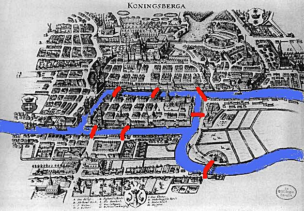
Given a graph $G=(V,E)$ , we usually use $n$ to denote the number of vertices $|V|$ and $m$ to denote the number of edges $|E|$ .

Important Note (Representations of graphs)

There are two common ways to represent a graph. Let $v_1,v_2,\ldots,v_n$ be some arbitrary ordering of the vertices. In the adjacency matrix representation, a graph is represented by an $n \times n$ matrix $A$ such that $A[i,j] = \begin{cases} 1 & \quad \text{if $\{v_i,v_j\} \in E$,}\\ 0 & \quad \text{otherwise.}\\ \end{cases}$ The adjacency matrix representation is not always the best representation of a graph. In particular, it is wasteful if the graph has very few edges. For such graphs, it can be preferable to use the adjacency list representation. In the adjacency list representation, you are given an array of size $n$ and the $i$ ’th entry of the array contains a pointer to a linked list of vertices that vertex $i$ is connected to via an edge.

Exercise (Max number of edges in a graph)

In an $n$ -vertex graph, what is the maximum possible value for the number of edges in terms of $n$ ?

Definition (Neighborhood of a vertex)

Let $G=(V,E)$ be a graph, and $e = \{u,v\} \in E$ be an edge in the graph. In this case, we say that $u$ and $v$ are neighbors or adjacent. We also say that $u$ and $v$ are incident to $e$ . For $v \in V$ , we define the neighborhood of $v$ , denoted $N(v)$ , as the set of all neighbors of $v$ , i.e. $N(v) = \{u : \{v,u\} \in E\}$ . The size of the neighborhood, $|N(v)|$ , is called the degree of $v$ , and is denoted by $\deg(v)$ .

Definition (

d

-regular graphs)

A graph $G = (V,E)$ is called $d$ -regular if every vertex $v \in V$ satisfies $\deg(v) = d$ .

Theorem (Handshake Theorem)

Let $G=(V,E)$ be a graph. Then $\sum_{v \in V} \deg(v) = 2m.$

Exercise (Application of Handshake Theorem)

Is it possible to have a party with 251 people in which everyone knows exactly 5 other people in the party?

Definition (Paths and cycles)

Let $G=(V,E)$ be a graph. A path of length $k$ in $G$ is a sequence of distinct vertices $v_0,v_1,\ldots,v_k$ such that $\{v_{i-1}, v_i\} \in E$ for all $i \in \{1,2,\ldots,k\}$ . In this case, we say that the path is from vertex $v_0$ to vertex $v_k$ (or that the path is between $v_0$ and $v_k$ ).

A cycle of length $k$ (also known as a $k$ -cycle) in $G$ is a sequence of vertices $v_0, v_1, \ldots, v_{k-1}, v_0$ such that $v_0, v_1, \ldots, v_{k-1}$ is a path, and $\{v_0,v_{k-1}\} \in E$ . In other words, a cycle is just a “closed” path. The starting vertex in the cycle is not important. So for example, $v_1, v_2, \ldots, v_{k-1},v_0,v_1$ would be considered the same cycle. Also, if we list the vertices in reverse order, we consider it to be the same cycle. For example, $v_0, v_{k-1}, v_{k-2} \ldots, v_1, v_0$ represents the same cycle as before.

A graph that contains no cycles is called acyclic.

Definition (Connected graph, connected component)

Let $G = (V,E)$ be a graph. We say that two vertices in $G$ are connected if there is a path between those two vertices. A connected graph $G$ is such that every pair of vertices in $G$ is connected.

A subset $S \subseteq V$ is called a connected component of $G$ if $G$ restricted to $S$ , i.e. the graph $G' = (S, E' = \{\{u,v\} \in E : u,v \in S\})$ , is a connected graph, and $S$ is disconnected from the rest of the graph (i.e. $\{u,v\} \not \in E$ when $u \in S$ and $v \not \in S$ ). Note that a connected graph is a graph with only one connected component.

Definition (Distance between vertices)

Let $G=(V,E)$ be a graph. The distance between vertices $u, v \in V$ , denoted $\text{dist}(u,v)$ , is defined to be the length of the shortest path between $u$ and $v$ . If $u = v$ , then $\text{dist}(u,v) = 0$ , and if $u$ and $v$ are not connected, then $\text{dist}(u,v)$ is defined to be $\infty$ .

Theorem (Min number of edges to connect a graph)

Let $G = (V,E)$ be a connected graph with $n$ vertices and $m$ edges. Then $m \geq n-1$ . Furthermore, $m = n-1$ if and only if $G$ is acyclic.

Definition (Tree, leaf, internal node)

A graph satisfying two of the following three properties is called a tree:

connected,
$m = n-1$ ,
acyclic.

A vertex of degree 1 in a tree is called a leaf. And a vertex of degree more than 1 is called an internal node.

Exercise (Equivalent definitions of a tree)

Show that if a graph has two of the properties listed in Definition (Tree, leaf, internal node), then it automatically has the third as well.

Exercise (A tree has at least 2 leaves)

Let $T$ be a tree with at least $2$ vertices. Show that $T$ must have at least $2$ leaves.

Exercise (Max degree is at most number of leaves)

Let $T$ be a tree with $L$ leaves. Let $\Delta$ be the largest degree of any vertex in $T$ . Prove that $\Delta \leq L$ .

Note (Root, parent, child, sibling, etc.)

Given a tree, we can pick an arbitrary node to be the root of the tree. In a rooted tree, we use “family tree” terminology: parent, child, sibling, ancestor, descendant, lowest common ancestor, etc. (We assume you are already familiar with these terms.) Level $i$ of a rooted tree denotes the set of all vertices in the tree at distance $i$ from the root.

Definition (Directed graph)

A directed graph $G$ is a pair $(V,A)$ , where

$V$ is a non-empty finite set called the set of vertices (or nodes),
$A$ is a finite set called the set of directed edges (or arcs), and every element of $A$ is a tuple $(u,v)$ for $u, v \in V$ . If $(u,v) \in A$ , we say that there is a directed edge from $u$ to $v$ . Note that $(u,v) \neq (v,u)$ unless $u = v$ .

Note (Drawing directed graphs)

Below is an example of how we draw a directed graph:

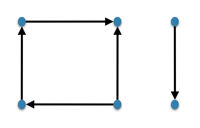
Definition (Neighborhood, out-degree, in-degree, sink, source)

Let $G = (V,A)$ be a directed graph. For $u \in V$ , we define the neighborhood of $u$ , $N(u)$ , as the set $\{v \in V : (u,v) \in A\}$ . The vertices in $N(u)$ are called the neighbors of $u$ . The out-degree of $u$ , denoted $\deg_\text{out}(u)$ , is $|N(u)|$ . The in-degree of $u$ , denoted $\deg_\text{in}(u)$ , is the size of the set $\{v \in V : (v,u) \in A\}$ . A vertex with out-degree 0 is called a sink. A vertex with in-degree 0 is called a source.

Note (Paths and cycles in directed graphs)

The notions of paths and cycles naturally extend to directed graphs. For example, we say that there is a path from $u$ to $v$ if there is a sequence of distinct vertices $u = v_0,v_1,\ldots,v_k = v$ such that $(v_{i-1}, v_i) \in A$ for all $i \in \{1,2,\ldots,k\}$ .

2. Graph Algorithms

Definition (Arbitrary-first search (AFS) algorithm)

The arbitrary-first search algorithm, denoted AFS, is the following generic algorithm for searching a given graph. Below, “bag” refers to an arbitrary data structure that allows us to add and retrieve objects. The algorithm, given a graph $G$ and some vertex $s$ in $G$ , traverses all the vertices in the connected componenet of $G$ containing $s$ .

$\begin{aligned} \hline\hline\\[-12pt] &\textbf{def}\;\; \text{AFS}(\langle \text{graph } G = (V,E), \; \text{vertex } s \in V \rangle):\\ &{\scriptstyle 1.}~~~~\texttt{Put $s$ into bag.}\\ &{\scriptstyle 2.}~~~~\texttt{While bag is non-empty:}\\ &{\scriptstyle 3.}~~~~~~~~\texttt{Pick an arbitrary vertex $v$ from bag.}\\ &{\scriptstyle 4.}~~~~~~~~\texttt{If $v$ is unmarked:}\\ &{\scriptstyle 5.}~~~~~~~~~~~~\texttt{Mark $v$.}\\ &{\scriptstyle 6.}~~~~~~~~~~~~\texttt{For each neighbor $w$ of $v$:}\\ &{\scriptstyle 7.}~~~~~~~~~~~~~~~~\texttt{Put $w$ into bag.}\\ \hline\hline\end{aligned}$

Note that when a vertex $w$ is added to the bag, it gets there because it is the neighbor of a vertex $v$ that has been just marked by the algorithm. In this case, we’ll say that $v$ is the parent of $w$ (and $w$ is the child of $v$ ). Explicitly keeping track of this parent-child relationship is convenient, so we modify the above algorithm to keep track of this information. Below, a tuple of vertices $(v,w)$ has the meaning that vertex $v$ is the parent of $w$ . The initial vertex $s$ has no parent, so we denote this situation by $(\perp, s)$ .

$\begin{aligned} \hline\hline\\[-12pt] &\textbf{def}\;\; \text{AFS}(\langle \text{graph } G = (V,E), \; \text{vertex } s \in V \rangle):\\ &{\scriptstyle 1.}~~~~\texttt{Put $(\perp, s)$ into bag.}\\ &{\scriptstyle 2.}~~~~\texttt{While bag is non-empty:}\\ &{\scriptstyle 3.}~~~~~~~~\texttt{Pick an arbitrary tuple $(p, v)$ from bag.}\\ &{\scriptstyle 4.}~~~~~~~~\texttt{If $v$ is unmarked:}\\ &{\scriptstyle 5.}~~~~~~~~~~~~\texttt{Mark $v$.}\\ &{\scriptstyle 6.}~~~~~~~~~~~~\text{parent}(v) = p.\\ &{\scriptstyle 7.}~~~~~~~~~~~~\texttt{For each neighbor $w$ of $v$:}\\ &{\scriptstyle 8.}~~~~~~~~~~~~~~~~\texttt{Put $(v,w)$ into bag.}\\ \hline\hline\end{aligned}$

Note (AFS-tree)

The parent pointers in the second algorithm above defines a tree, rooted at $s$ , spanning all the vertices in the connected component of the initial vertex $s$ . We’ll call this the tree induced by the search algorithm. Having a visualization of this tree and how the algorithm traverses the vertices in the tree can be a useful way to understand how the algorithm works. Below, we will actualize AFS by picking specific data structures for the bag. We’ll then comment on the properties of the induced tree.

Note (Traversing all the vertices in the graph)

Note that AFS( $G$ , $s$ ) visits all the vertices in the connected component that $s$ is a part of. If we want to traverse all the vertices in the graph, and the graph has multiple connected components, then we can do: $\begin{aligned} \hline\hline\\[-12pt] &\textbf{def}\;\; \text{AFS2}(\langle \text{graph } G = (V,E) \rangle):\\ &{\scriptstyle 1.}~~~~\texttt{For $v$ not marked as visited:}\\ &{\scriptstyle 2.}~~~~~~~~\texttt{Run } \text{AFS}(\langle G, v \rangle)\\ \hline\hline\end{aligned}$

Definition (Breadth-first search (BFS) algorithm)

The breadth-first search algorithm, denoted BFS, is AFS where the bag is chosen to be a queue data structure.

Note (Running time of BFS)

The running time of BFS( $G,s$ ) is $O(m)$ , where $m$ is the number of edges of the input graph. If we do a BFS for each connected component, the total running time is $O(m+n)$ , where $n$ is the number of vertices. (We are assuming the graph is given as an adjacency list.)

Note (BFS-tree)

The induced tree of BFS is called the BFS-tree. In this tree, vertices $v$ at level $i$ of the tree are exactly those vertices with $\text{dist}(s,v) = i$ . BFS first traverses vertices at level 1, then level 2, then level 3, and so on. This is why the name of the algorithm is breadth-first search.

Assuming $G$ is connected, we can think of $G$ as the BFS-tree, plus, the “extra” edges in $G$ that are not part of the BFS-tree. Observe that an extra edge is either between two vertices at the same level, or is between two vertices at consecutive levels in the BFS-tree.

Definition (Depth-first search (DFS) algorithm)

The depth-first search algorithm, denoted DFS, is AFS where the bag is chosen to be a stack data structure.

Note (Recursive DFS)

There is a natural recursive representation of the DFS algorithm, as follows. $\begin{aligned} \hline\hline\\[-12pt] &\textbf{def}\;\; \text{DFS}(\langle \text{graph } G = (V,E), \; \text{vertex } s \in V \rangle):\\ &{\scriptstyle 1.}~~~~\texttt{Mark $s$.}\\ &{\scriptstyle 2.}~~~~\texttt{For each neighbor $v$ of $s$:}\\ &{\scriptstyle 3.}~~~~~~~~\texttt{If $v$ is unmarked:}\\ &{\scriptstyle 4.}~~~~~~~~~~~~\texttt{Run } \text{DFS}(\langle G, v \rangle).\\ \hline\hline\end{aligned}$

Note (Running time of DFS)

The running time of DFS( $G,s$ ) is $O(m)$ , where $m$ is the number of edges of the input graph. If we do a DFS for each connected component, the total running time is $O(m+n)$ , where $n$ is the number of vertices. (We are assuming the graph is given as an adjacency list.)

Note (DFS-tree)

The induced tree of DFS is called the DFS-tree. At a high level, DFS goes as deep as it can in the DFS-tree until it cannot go deeper, in which case it backtracks until it can go deeper again. This is why the name of the algorithm is depth-first search.

Assuming $G$ is connected, we can think of $G$ as the DFS-tree, plus, the “extra” edges in $G$ that are not part of the DFS-tree. Observe that an extra edge must be between two vertices such that one is the ancestor of the other in the DFS-tree.

Note (Search algorithms on directed graphs)

The search algorithms presented above can be applied to directed graphs as well.

Definition (Minimum spanning tree (MST) problem)

In the minimum spanning tree problem, the input is a connected undirected graph $G = (V,E)$ together with a cost function $c : E \to \mathbb R^+$ . The output is a subset of the edges of minimum total cost such that, in the graph restricted to these edges, all the vertices of $G$ are connected. For convenience, we’ll assume that the edges have unique edge costs, i.e. $e \neq e' \implies c(e) \neq c(e')$ .

Note (Unique edges costs imply unique MST)

With unique edge costs, the minimum spanning tree is unique.

Theorem (MST cut property)

Suppose we are given an instance of the MST problem. For any non-trivial subset $S \subseteq V$ , let $e^* = \{u^*, v^*\}$ be the cheapest edge with the property that $u^* \in S$ and $v^* \in V \backslash S$ . Then $e^*$ must be in the minimum spanning tree.

Theorem (Jarník-Prim algorithm for MST)

There is an algorithm that solves the MST problem in polynomial time.

Exercise (MST with negative costs)

Suppose an instance of the Minimum Spanning Tree problem is allowed to have negative costs for the edges. Explain whether we can use the Jarník-Prim algorithm to compute the minimum spanning tree in this case.

Exercise (Maximum spanning tree)

Consider the problem of computing the maximum spanning tree, i.e., a spanning tree that maximizes the sum of the edge costs. Explain whether the Jarník-Prim algorithm solves this problem if we modify it so that at each iteration, the algorithm chooses the edge between $V'$ and $V\backslash V'$ with the maximum cost.

3. Check Your Understanding

Problem

What is the maximum possible value for the number of edges in an undirected graph (no self-loops, no multi-edges) in terms of $n$ , the number of vertices?
How do you prove the Handshake Theorem?
What is the definition of a tree?
True or false: If $G = (V, E)$ is a tree, then for any $u, v \in V$ , there exists a unique path from $u$ to $v$ .
True or false: For a graph $G = (V, E)$ , if for any $u, v \in V$ there exists a unique path from $u$ to $v$ , then $G$ is a tree.
True or false: If a graph on $n$ vertices has $n-1$ edges, then it must be acyclic.
True or false: If a graph on $n$ vertices has $n-1$ edges, then it must be connected.
True or false: If a graph on $n$ vertices has $n-1$ edges, then it must be a tree.
True or false: A tree with $n \geq 2$ vertices can have a single leaf.
What is the minimum number of edges possible in a connected graph with $n$ vertices? And what are the high-level steps of the proof?
True or false: An acyclic graph with $k$ connected components has $n-k$ edges.
True or false: For every tree on $n$ vertices, $\sum_{v \in V} \deg(v)$ has exactly the same value.
True or false: Let $G$ be a $5$ -regular graph (i.e. a graph in which every vertex has degree exactly $5$ ). It is possible that $G$ has $15251$ edges.
True or false: There exists $n_0 \in \mathbb{N}$ such that for all $n > n_0$ , there is a graph $G$ with $n$ vertices that is $3$ -regular.
What is the difference between BFS and DFS?
True or false: DFS algorithm runs in $O(n)$ time for a connected graph, where $n$ is the number of vertices of the input graph.
Explain why the running time of BFS and DFS is $O(m+n)$ ; in particular where does the $m$ come from and where does the $n$ come from?
What is the MST cut property?
Consider the following “proof” of the MST cut property:

Assume for the sake of contradiction that the MST $T$ does not contain the edge $e^*$ . Since $T$ is a spanning tree, it must contain an edge $e'$ with one endpoint in $S$ and one endpoint not in $S$ . Since $e^*$ is the cheapest edge with this property, it follows that $T^* = (T \backslash \{e'\}) \cup \{e^*\}$ is a spanning tree that is cheaper than $T$ , a contradiction.

Expose the flaw in this argument by giving a specific example where it fails.
Explain at a high-level how the Jarník-Prim algorithm works.
True or false: Suppose a graph has $2$ edges with the same cost. Then there are at least $2$ minimum spanning trees of the graph.

4. High-Order Bits

Important Note

Here are the important things to keep in mind from this chapter.

There are many definitions in this chapter. This is unfortunately inevitable in order to effectively communicate with each other. On the positive side, the definitions are often very intuitive and easy to guess. It is important that you are comfortable with all the definitions.
In the first section of the chapter, we see a few proof techniques on graphs: degree counting arguments, induction arguments, the trick of removing all the edges of graph and adding them back in one by one. Make sure you understand these techniques well. They can be very helpful when you are coming up with proofs yourself.
The second section of the chapter contains some well-known graph algorithms. These algorithms are quite fundamental, and you may have seen them (or will see them) in other courses. Make sure you understand at a high level how the algorithms work. The implementation details are not important in this course.

Matchings in Graphs

1. Maximum Matchings

Definition (Matching – maximum, maximal, perfect)

A matching in a graph $G=(V,E)$ is a subset of the edges that do not share an endpoint. A maximum matching in $G$ is a matching with the maximum number of edges among all possible matchings. A maximal matching is a matching with the property that if we add any other edge to the matching, it is no longer a matching. A perfect matching is a matching that covers all the vertices of the graph.

Note (Size of a matching)

The size of a matching $M$ refers to the number of edges in the matching, and is denoted by $|M|$ . Note that this coincides with the size of the set that $M$ represents.

Definition (Maximum matching problem)

In the maximum matching problem the input is an undirected graph $G=(V,E)$ and the output is a maximum matching in $G$ .

Definition (Augmenting path)

Let $G = (V,E)$ be a graph and let $M \subseteq E$ be a matching in $G$ . An augmenting path in $G$ with respect to $M$ is a path such that

the path is an alternating path, which means that the edges in the path alternate between being in $M$ and not in $M$ ,
the first and last vertices in the path are not a part of the matching $M$ .

Note (Edge cases for augmenting paths)

An augmenting path does not need to contain all the edges in $M$ . It is also possible that it does not contain any of the edges of $M$ . A single edge $\{u, v\}$ , where $u$ is not matched and $v$ is not matched, is an augmenting path.

Theorem (Characterization for maximum matchings)

Let $G=(V,E)$ be a graph. A matching $M \subseteq E$ is maximum if and only if there is no augmenting path in $G$ with respect to $M$ .

Exercise (Graphs with max degree at most 2)

Let $G = (V,E)$ be a graph such that all vertices have degree at most $2$ . Then prove that every connected component of $G$ is either a path or a cycle (where we count an isolated vertex as a path of length 0).

Exercise (A tree can have at most one perfect matching)

Show that a tree can have at most one perfect matching.

2. Bipartite Graphs

Definition (Bipartite graph)

A graph $G = (V,E)$ is called bipartite if there is a partition of $V$ into sets $X$ and $Y$ such that all the edges in $E$ have one endpoint in $X$ and the other in $Y$ . Sometimes the bipartition is given explicitly and the graph is denoted by $G = (X, Y, E)$ .

Definition (

k

-colorable graphs)

Let $G = (V,E)$ be a graph. Let $k \in \mathbb{N}^+$ . A $k$ -coloring of $V$ is just a map $\chi : V \to C$ where $C$ is a set of cardinality $k$ . (Usually the elements of $C$ are called colors. If $k = 3$ then $C = \{\text{red},\text{green},\text{blue}\}$ is a popular choice. If $k$ is large, we often just call the “colors” $1,2, \dots, k$ .) A $k$ -coloring is said to be legal for $G$ if every edge in $E$ is bichromatic, meaning that its two endpoints have different colors. (I.e., for all $\{u,v\} \in E$ it is required that $\chi(u)\neq\chi(v)$ .) Finally, we say that $G$ is $k$ -colorable if it has a legal $k$ -coloring.

Note (2-colorability is equivalent to bipartiteness)

A graph $G=(V,E)$ is bipartite if and only if it is $2$ -colorable. The $2$ -coloring corresponds to partitioning the vertex set $V$ into $X$ and $Y$ such that all the edges have one endpoint in $X$ and the other in $Y$ .

Theorem (Characterization of bipartite graphs)

A graph is bipartite if and only if it contains no odd-length cycles.

Theorem (Finding a maximum matching in bipartite graphs)

There is a polynomial time algorithm to solve the maximum matching problem in bipartite graphs.

Note (Finding a maximum matching in non-bipartite graphs)

The high-level algorithm above presented in the proof of Theorem (Finding a maximum matching in bipartite graphs) is in fact applicable to general (not necessarily bipartite) graphs. However, the step of finding an augmenting path with respect to a matching turns out to be much more involved, and therefore we do not cover it in this chapter. See https://en.wikipedia.org/wiki/Blossom_algorithm if you would like to learn more.

3. Bonus: Hall’s Theorem

Theorem (Hall’s Theorem)

Let $G = (X,Y,E)$ be a bipartite graph. For a subset $S$ of the vertices, let $N(S) = \bigcup_{v \in S} N(v)$ . Then $G$ has a matching covering all the vertices in $X$ if and only if for all $S \subseteq X$ , we have $|S| \leq |N(S)|$ .

Corollary (Characterization of bipartite graphs with perfect matchings)

Let $G = (X,Y,E)$ be a bipartite graph. Then $G$ has a perfect matching if and only if $|X| = |Y|$ and for any $S \subseteq X$ , we have $|S| \leq |N(S)|$ .

Note (Hall’s Theorem when the two parts have equal size)

Sometimes people call the above corollary Hall’s Theorem.

Exercise (Practice with perfect matchings)

Let $G$ be a bipartite graph on $2n$ vertices such that every vertex has degree at least $n$ . Prove that $G$ must contain a perfect matching.
Let $G = (X,Y,E)$ be a bipartite graph with $|X| = |Y|$ . Show that if $G$ is connected and every vertex has degree at most $2$ , then $G$ must contain a perfect matching.

4. Check Your Understanding

Problem

True or false: A maximum matching is a maximal matching.
True or false: A perfect matching is a maximum matching.
True or false: There exist graphs with more than one perfect matching.
How many perfect matchings are there in a complete bipartite graph (all possible edges are present) where both sides of the bipartition contain exactly $n$ vertices?
Suppose a graph with $n$ vertices has a perfect matching. What is the size of the perfect matching?
What is the definition of an augmenting path?
True or false: A single edge $\{u, v\}$ , where $u$ is not matched and $v$ is not matched, is an augmenting path.
True or false: Given a matching $M$ , there can be at most one augmenting path with respect to $M$ .
True or false: A matching $M$ in a non-bipartite graph $G$ is maximum if and only if there is no augmenting path with respect to $M$ .
Describe the high-level steps of a polynomial-time algorithm for finding a maximum matching in a graph.
Describe a polynomial-time algorithm that given a bipartite graph and a matching in the graph, determines if an augmenting path exists with respect to the matching.
True or false: The graph below is bipartite.
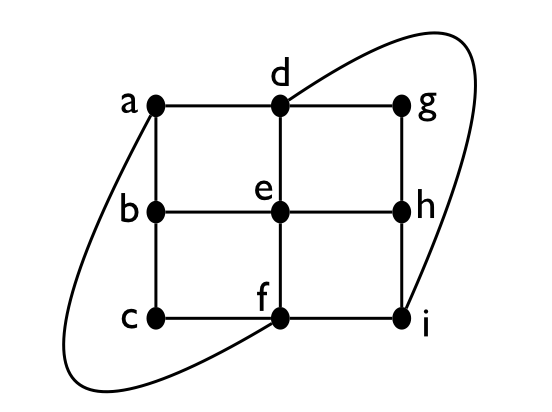
True or false: If a graph is $k$ -colorable, then it is $(k+1)$ -colorable.
True or false: A graph which is not bipartite must contain an odd-length cycle.
Explain how one can $2$ -color a graph that does not contain an odd-length cycle.
Describe a polynomial-time algorithm to determine if an input undirected graph is bipartite or not.
How do you prove that a tree has at most one perfect matching?
True or false: Any graph with more than one perfect matching must contain a cycle.
In this chapter we saw the definition of a bipartite graph. We can think of a bipartite graph as a special case of a $k$ -partite graph where $k = 2$ . How would you define the general notion of a $k$ -partite graph, and how does it relate to the colorability of the graph?

5. High-Order Bits

Important Note

Here are the important things to keep in mind from this chapter.

As always, all the definitions in this chapter are important (matchings, augmenting path, bipartite graph, $k$ -coloring of a graph).
Theorem (Characterization of bipartite graphs) gives an important characterization for bipartite graphs. Make sure to understand its proof.
Theorem (Characterization for maximum matchings) gives an important characterization for maximum matchings. The proof is one of the harder proofs we have done in the course so far. A good understanding of the proof is expected and important since it will help you raise your level of mathematical maturity.
Make sure to understand how we can use Theorem (Characterization for maximum matchings) to come up with an algorithm for finding a maximum matching in a graph.

Stable Matchings

1. Stable Matching Problem

Definition (Stable matching problem)

An instance of the stable matching problem is a tuple of sets $(X, Y)$ with $|X| = |Y|$ , and a preference list for each element of $X$ and $Y$ . A preference list for an element in $X$ is an ordering of the elements in $Y$ , and a preference list for an element in $Y$ is an ordering of the elements of $X$ . Below is an example of an instance of the stable matching problem:

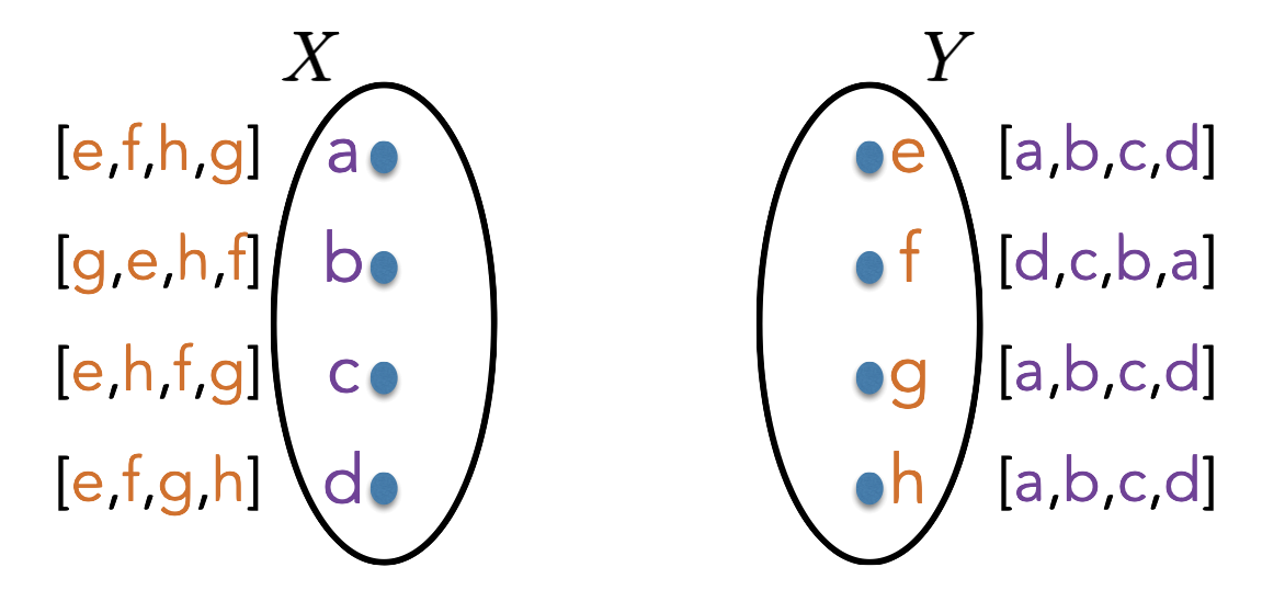
The output of the stable matching problem is a stable matching, which is a subset $S$ of $\{(x, y) : x \in X, y \in Y\}$ with the following properties:

The matching is a perfect matching, which means every $x \in X$ and every $y \in Y$ appear exactly once in $S$ . If $(x,y) \in S$ , we say $x$ and $y$ are matched.
There are no unstable pairs. A pair $(x,y)$ where $x \in X$ and $y \in Y$ is called unstable if $(x,y) \not \in S$ , but they both prefer each other to the elements they are matched to.

Theorem (Gale-Shapley proposal algorithm)

There is a polynomial time algorithm which, given an instance of the stable matching problem, always returns a stable matching.

Definition (Best and worst valid partners)

Consider an instance of the stable matching problem. We say that $x \in X$ is a valid partner of $y \in Y$ (or $y$ is a valid partner of $x$ ) if there is some stable matching in which $x$ and $y$ are matched. For $z \in X \cup Y$ , we define the best valid partner of $z$ , denoted $\text{best}(z)$ , to be the highest ranked valid partner of $z$ . Similarly, we define the worst valid partner of $z$ , denoted $\text{worst}(z)$ , to be the lowest ranked valid partner of $z$ .

Theorem (Gale-Shapley is

X

-optimal)

The Gale-Shapley algorithm always matches $x \in X$ with its best valid partner, i.e., it returns $\{(x, \text{best}(x)): x \in X \}$ .

Note (Interesting consequence of Gale-Shapley)

Note that it is not a priori clear at all that $\{(x, \text{best}(x)): x \in X \}$ would be a matching, not to mention a stable matching.

Exercise (Gale-Shapley is

Y

-pessimal)

Show that the Gale-Shapley algorithm always matches $y \in Y$ with its worst valid partner, i.e., it returns $\{(\text{worst}(y), y): y \in Y \}$ .

Exercise (Is there a unique stable matching?)

Give a polynomial time algorithm that determines if a given instance of the stable matching problem has a unique solution or not.

Exercise (Identical preferences)

Suppose we are given an instance of the stable matching problem in which all $x \in X$ have identical preference lists, and all $y \in Y$ have identical preference lists. Prove or disprove: there is only one stable matching for such an instance.

Exercise (Stable roommates problem)

Consider the following variant of the stable matching problem. The input is a set of $n$ people, where $n$ is even. Each person has a preference list that includes every other person. The goal is to find a stable matching. Give an example to show that a stable matching does not always exist.

Exercise (Soulmates)

Call $x \in X$ and $y \in Y$ “soulmates” if they are paired with each other in every stable matching.

Given $x \in X$ and $y \in Y$ , design a polynomial-time algorithm to determine if they are soulmates.
Give a polynomial time algorithm to determine if an instance of the stable matching problem has a unique stable matching.

2. Check Your Understanding

Problem

What is the definition of a stable matching?
Give an example of a stable matching problem instance that has at least two stable matchings.
What are the definitions of valid partner, best valid partner, and worst valid partner?
Describe the Gale-Shapley algorithm.
True or false: In any instance of the stable matching problem, a stable matching always exists.
True or false: In any instance of the stable matching problem, there is at most one stable matching.
What does it mean for a matching to be $X$ -optimal?
What does it mean for a matching to be $X$ -pessimal?
True or false: The Gale-Shapley algorithm can output different matchings based on the order of the companies proposing.
True or false: For every stable matching instance, the $X$ -optimal and $Y$ -optimal stable matchings differ in at least one pairing.
True or false: Given an instance of the stable matching problem, it is not possible for two companies to have the same best valid partner.
True or false: If the Gale-Shapley algorithm ends up pairing $x \in X$ with its worst possible partner $y \in Y$ , then $x$ and $y$ must be paired/matched in all stable matchings.

3. High-Order Bits

Important Note

Your main goal should be to really understand the stable matching problem, the Gale-Shapley algorithm that solves the stable matching problem, and the proof of correctness of the algorithm.
Best and worst valid partners are important notions. Make sure you understand what they mean and how they relate to the Gale-Shapley algorithm’s output.

Polynomial-Time Reductions

1. Problems of Interest

Definition (

k

-Coloring problem)

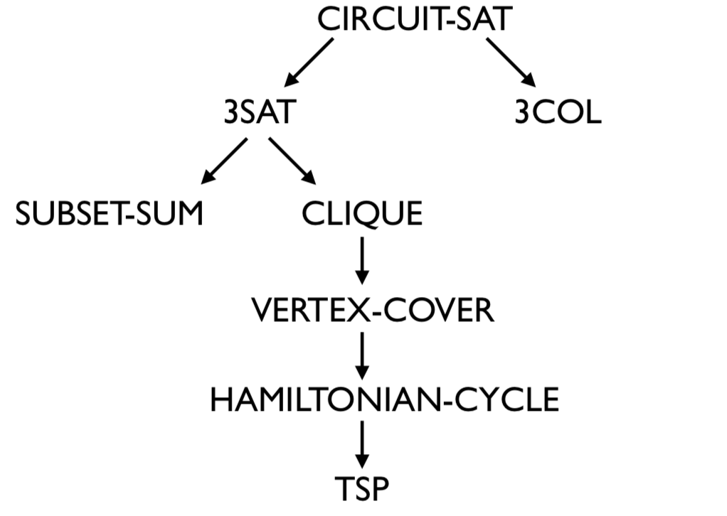
In the $k$ -coloring problem, the input is an undirected graph $G=(V,E)$ , and the output is True if and only if the graph is $k$ -colorable (see Definition ( $k$ -colorable graphs)). We denote this problem by $k\text{COL}$ . The corresponding language is $\{\langle G \rangle: \text{$G$ is a $k$-colorable graph}\}.$

Definition (Clique problem)

Let $G = (V,E)$ be an undirected graph. A subset $S$ of the vertices is called a clique if for all $u, v \in S$ with $u \neq v$ , $\{u,v\} \in E$ . We say that $G$ contains a $k$ -clique if there is a subset of the vertices of size $k$ that forms a clique.

In the clique problem, the input is an undirected graph $G=(V,E)$ and a number $k \in \mathbb N^+$ , and the output is True if and only if the graph contains a $k$ -clique. We denote this problem by $\text{CLIQUE}$ . The corresponding language is $\{\langle G, k \rangle: \text{$G$ is a graph, $k \in \mathbb N^+$, $G$ contains a $k$-clique}\}.$

Definition (Independent set problem)

Let $G = (V,E)$ be an undirected graph. A subset of the vertices is called an independent set if there is no edge between any two vertices in the subset. We say that $G$ contains an independent set of size $k$ if there is a subset of the vertices of size $k$ that forms an independent set.

In the independent set problem, the input is an undirected graph $G=(V,E)$ and a number $k \in \mathbb N^+$ , and the output is True if and only if the graph contains an independent set of size $k$ . We denote this problem by $\text{IS}$ . The corresponding language is $\{\langle G, k \rangle: \text{$G$ is a graph, $k \in \mathbb N^+$, $G$ contains an independent set of size $k$}\}.$

Note (Unary NOT, binary AND, binary OR)

We denote by $\neg$ the unary NOT operation, by $\wedge$ the binary AND operation, and by $\vee$ the binary OR operation. In particular, we can write the truth tables of these operations as follows:

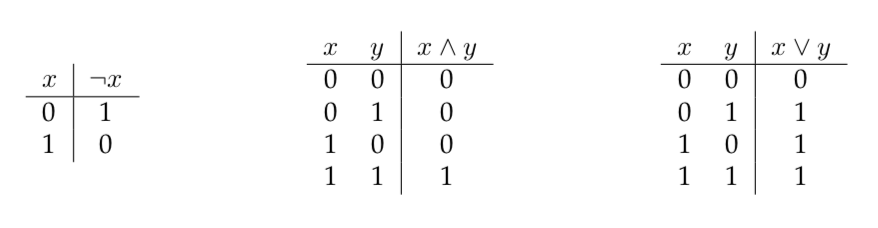
Definition (Boolean satisfiability problem)

Let $x_1,\ldots,x_n$ be Boolean variables, i.e., variables that can be assigned True or False. A literal refers to a Boolean variable or its negation. A clause is an “OR” of literals. For example, $x_1 \vee \neg x_3 \vee x_4$ is a clause. A Boolean formula in conjunctive normal form (CNF) is an “AND” of clauses. For example, $(x_1 \vee \neg x_3) \wedge (x_2 \vee x_2 \vee x_4) \wedge (x_1 \vee \neg x_1 \vee \neg x_5) \wedge x_4$ is a CNF formula. We say that a Boolean formula is a satisfiable formula if there is a truth assignment (which can also be viewed as a $0/1$ assignment) to the Boolean variables that makes the formula evaluate to true (or $1$ ).

In the CNF satisfiability problem, the input is a CNF formula, and the output is True if and only if the formula is satisfiable. We denote this problem by $\text{SAT}$ . The corresponding language is $\{\langle \varphi \rangle: \text{$\varphi$ is a satisfiable CNF formula}\}.$ In a variation of $\text{SAT}$ , we restrict the input formula such that every clause has exactly 3 literals (we call such a formula a 3CNF formula). For instance, the following is a 3CNF formula: For example, $(x_1 \vee \neg x_3 \vee x_4) \wedge (x_2 \vee x_2 \vee x_4) \wedge (x_1 \vee \neg x_1 \vee \neg x_5) \wedge (\neg x_2 \vee \neg x_3 \vee \neg x_3)$ This variation of the problem is denoted by $\text{3SAT}$ .

Definition (Boolean circuit)

A Boolean circuit with $n$ -input variables ( $n \geq 0$ ) is a directed acyclic graph with the following properties. Each node of the graph is called a gate and each directed edge is called a wire. There are $5$ types of gates that we can choose to include in our circuit: AND gates, OR gates, NOT gates, input gates, and constant gates. There are 2 constant gates, one labeled $0$ and one labeled $1$ . These gates have in-degree/fan-in $0$ . There are $n$ input gates, one corresponding to each input variable. These gates also have in-degree/fan-in $0$ . An AND gate corresponds to the binary AND operation $\wedge$ and an OR gate corresponds to the binary OR operation $\vee$ . These gates have in-degree/fan-in $2$ . A NOT gate corresponds to the unary NOT operation $\neg$ , and has in-degree/fan-in $1$ . One of the gates in the circuit is labeled as the output gate. Gates can have out-degree more than $1$ , except for the output gate, which has out-degree $0$ .

For each 0/1 assignment to the input variables, the Boolean circuit produces a one-bit output. The output of the circuit is the output of the gate that is labeled as the output gate. The output is calculated naturally using the truth tables of the operations corresponding to the gates. The input-output behavior of the circuit defines a function $f:\{0,1\}^n \to \{0,1\}$ and in this case, we say that $f$ is computed by the circuit.

Definition (Circuit satisfiability problem)

A satisfiable circuit is such that there is 0/1 assignment to the input gates that makes the circuit output 1. In the circuit satisfiability problem, the input is a Boolean circuit, and the output is True if and only if the circuit is satisfiable. We denote this problem by $\text{CIRCUIT-SAT}$ . The corresponding language is $\{\langle C \rangle: \text{$C$ is a Boolean circuit that is satisfiable}\}.$

Note (Names of decision problems and languages)

The name of a decision problem above refers both to the decision problem and the corresponding language.

Note (Inputs of decision problems)

Recall that in all the decision problems above, the input is an arbitrary word in $\Sigma^*$ . If the input does not correspond to a valid encoding of an object expected as input (e.g. a graph in the case of $k$ COL), then those inputs are rejected (i.e., they are not in the corresponding language).

Note (Exponential-time algorithms for the decision problems above)

All the problems defined above are decidable and have exponential-time algorithms solving them.

2. Cook and Karp Reductions

Note (Cook reduction: Polynomial-time (Turing) reduction)

Fix some alphabet $\Sigma$ . Let $A$ and $B$ be two languages. We say that $A$ polynomial-time reduces to $B$ , written $A \leq^PB$ , if there is a polynomial-time decider for $A$ that uses a decider for $B$ as a black-box subroutine. Polynomial-time reductions are also known as Cook reductions, named after Stephen Cook.

Note (Polynomial-time reductions and

\mathsf{P}

)

Suppose $A \leq^PB$ . Observe that if $B \in \mathsf{P}$ , then $A \in \mathsf{P}$ . Equivalently, taking the contrapositive, if $A \not \in \mathsf{P}$ , then $B \not \in \mathsf{P}$ . So when $A \leq^PB$ , we think of $B$ as being at least as hard as $A$ with respect to polynomial-time decidability.

Note (Transitivity of Cook reductions)

Note that if $A \leq^PB$ and $B \leq^PC$ , then $A \leq^PC$ .

Definition (Karp reduction: Polynomial-time mapping reduction)

Let $A$ and $B$ be two languages. Suppose that there is a polynomial-time computable function (also called a polynomial-time transformation) $f: \Sigma^* \to \Sigma^*$ such that $x \in A$ if and only if $f(x) \in B$ . Then we say that there is a polynomial-time mapping reduction (or a Karp reduction, named after Richard Karp) from $A$ to $B$ , and denote it by $A \leq_m^PB$ .

Important Note (Steps to establish a Karp reduction)

To show that there is a Karp reduction from $A$ to $B$ , you need to do the following things.

Present a computable function $f: \Sigma^* \to \Sigma^*$ .
Show that $x \in A \implies f(x) \in B$ .
Show that $x \not \in A \implies f(x) \not \in B$ (it is usually easier to argue the contrapositive).
Show that $f$ can be computed in polynomial time.

In picture, the transformation $f$ looks as follows.

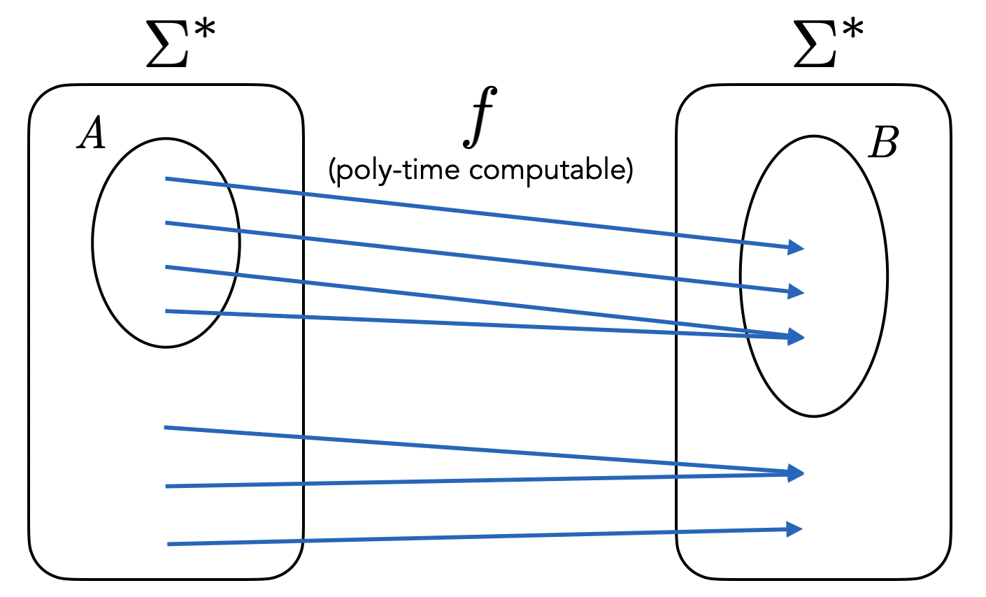
Note that $f$ need not be injective and it need not be surjective.

Important Note (Mapping reductions vs Turing reductions)

Recall that a mapping reduction is really a special kind of a Turing reduction. In particular, if there is a mapping reduction from language $A$ to language $B$ , then one can construct a regular (Turing) reduction from $A$ to $B$ . We explain this below as a reminder.

To establish a Turing reduction from $A$ to $B$ , we need to show how we can come up with a decider $M_A$ for $A$ given that we have a decider $M_B$ for $B$ . Now suppose we have a mapping reduction from $A$ to $B$ . This means we have a computable function $f$ as in the definition of a mapping reduction. This $f$ then allows us to build $M_A$ as follows. Given any input $x$ , first feed $x$ into $f$ , and then feed the output $y = f(x)$ into $M_B$ . The output of $M_A$ is the output of $M_B$ . We illustrate this construction with the following picture.

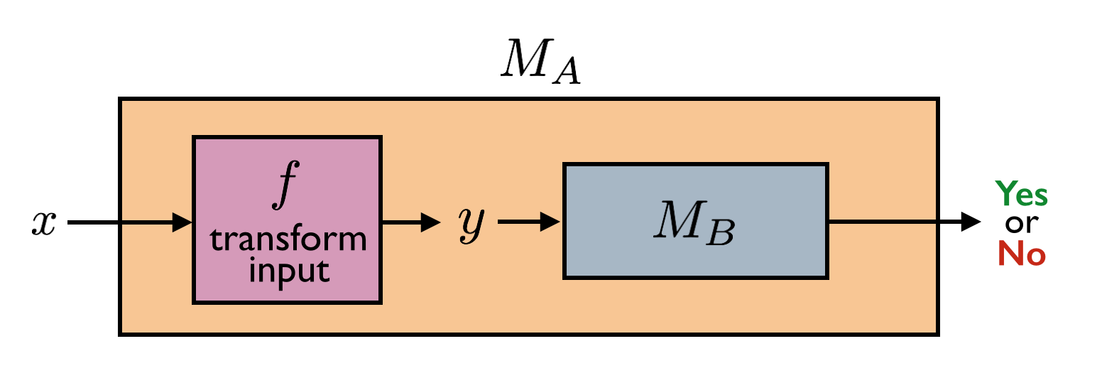
Take a moment to verify that this reduction from $A$ to $B$ is indeed correct given the definition of $f$ .

Even though a mapping reduction can be viewed as a regular (Turing) reduction, not all reductions are mapping reductions.

Theorem (CLIQUE reduces to IS)

$\text{CLIQUE} \leq_m^P\text{IS}$ .

Exercise (IS reduces to CLIQUE)

How can you modify the above reduction to show that $\text{IS} \leq_m^P\text{CLIQUE}$ ?

Exercise (Hamiltonian path reductions)

Let $G=(V,E)$ be a graph. A Hamiltonian path in $G$ is a path that visits every vertex of the graph exactly once. The HAMPATH problem is the following: given a graph $G=(V,E)$ , output True if it contains a Hamiltonian path, and output False otherwise.

Let $L = \{\langle G, k \rangle : \text{$G$ is a graph, $k \in \mathbb N$, $G$ has a path of length $k$}\}$ . Show that $\text{HAMPATH}\leq_m^PL$ .
Let $K = \{\langle G, k \rangle : \text{$G$ is a graph, $k \in \mathbb N$, $G$ has a spanning tree with $\leq k$ leaves}\}$ . Show that $\text{HAMPATH}\leq_m^PK$ .

Theorem (CIRCUIT-SAT reduces to 3COL)

$\text{CIRCUIT-SAT}\leq_m^P3\text{COL}$ .

Exercise (Transitivity of Karp reductions)

Show that if $A \leq_m^PB$ and $B \leq_m^PC$ , then $A \leq_m^PC$ .

3. Hardness and Completeness

Definition (

\mathcal{C}

-hard,

\mathcal{C}

-complete)

Let $\mathcal{C}$ be a set of languages containing $\mathsf{P}$ .

We say that $L$ is $\mathcal{C}$ -hard (with respect to Cook reductions) if for all languages $K \in \mathcal{C}$ , $K \leq^PL$ .
(With respect to polynomial time decidability, a $\mathcal{C}$ -hard language is at least as “hard” as any language in $\mathcal{C}$ .)
We say that $L$ is $\mathcal{C}$ -complete if $L$ is $\mathcal{C}$ -hard and $L \in \mathcal{C}$ .
(A $\mathcal{C}$ -complete language represents the “hardest” language in $\mathcal{C}$ with respect to polynomial time decidability.)

Note (

\mathcal{C}

-completeness and

\mathsf{P}

)

Suppose $L$ is $\mathcal{C}$ -complete. Then observe that $L \in \mathsf{P}\Longleftrightarrow \mathcal{C}= \mathsf{P}$ .

Note (

\mathcal{C}

-hardness with respect to Cook and Karp reductions)

Above we have defined $\mathcal{C}$ -hardness using Cook reductions. In literature, however, they are often defined using Karp reductions, which actually leads to a different notion of $\mathcal{C}$ -hardness. There are good reasons to use this restricted form of reductions. More advanced courses may explore some of these reasons.

4. Check Your Understanding

Problem

What is a Cook reduction? What is a Karp reduction? What is the difference between the two?
Explain why every Karp reduction can be viewed as a Cook reduction.
Explain why every Cook reduction cannot be viewed as a Karp reduction.
True or false: $\Sigma^* \leq_m^P\varnothing$ .
True or false: For languages $A$ and $B$ , $A \leq_m^PB$ if and only if $B \leq_m^PA$ .
Define the complexity class $\mathsf{P}$ .
True or false: The language $\text{251CLIQUE} = \{\langle G \rangle : \text{ $G$ is a graph containing a clique of size 251}\}$ is in $\mathsf{P}$ .
True or false: Let $L, K \subseteq \Sigma^*$ be two languages. Suppose there is a polynomial-time computable function $f : \Sigma^*\to\Sigma^*$ such that $x\in L$ iff $f(x)\notin K$ . Then $L$ Cook-reduces to $K$ .
True or false: There is a Cook reduction from 3SAT to HALTS.
For a complexity class $\mathcal{C}$ containing $\mathsf{P}$ , define what it means to be $\mathcal{C}$ -hard.
For a complexity class $\mathcal{C}$ containing $\mathsf{P}$ , define what it means to be $\mathcal{C}$ -complete.
Suppose $L$ is $\mathcal{C}$ -complete. Then argue why $L \in \mathsf{P}\Longleftrightarrow \mathcal{C}= \mathsf{P}$ .

5. High-Order Bits

Important Note

There are two very important notions of reductions introduced in this chapter: Cook reductions and Karp reductions. Make sure you understand the similarities and differences between them. And make sure you are comfortable presenting and proving the correctness of reductions. This is the main goal of the chapter.
The chapter concludes with a couple of important definitions: $\mathcal{C}$ -hardness, $\mathcal{C}$ -completeness. We present these definitions in this chapter as they are closely related to reductions. However, we will make use of these definitions in the next chapter after we introduce the complexity class $\mathsf{NP}$ . For now, make sure you understand the definitions and also Note ( $\mathcal{C}$ -completeness and $\mathsf{P}$ ).

Non-Deterministic Polynomial Time

1. Non-Deterministic Polynomial Time NP

Definition (Non-deterministic polynomial time, complexity class

\mathsf{NP}

)

Fix some alphabet $\Sigma$ . We say that a language $L$ can be decided in non-deterministic polynomial time if there exists

a polynomial-time decider TM $V$ that takes two strings as input, and
a constant $k > 0$ ,

such that for all $x \in \Sigma^*$ :

if $x \in L$ , then there exists $u \in \Sigma^*$ with $|u| \leq |x|^k$ such that $V(x,u)$ accepts,
if $x \not \in L$ , then for all $u \in \Sigma^*$ , $V(x,u)$ rejects.

If $x \in L$ , a string $u$ that makes $V(x,u)$ accept is called a proof (or certificate) of $x$ being in $L$ . The TM $V$ is called a verifier for $L$ .

We denote by $\mathsf{NP}$ the set of all languages which can be decided in non-deterministic polynomial time.

Proposition (3COL is in

\mathsf{NP}

)

$\text{3COL} \in \mathsf{NP}$ .

Note (Steps to show a languages is in

\mathsf{NP}

)

Showing that a language $L$ is in $\mathsf{NP}$ involves the following steps:

Present a TM $V$ (that takes two inputs $x$ and $u$ ).
Argue that $V$ has polynomial running time.
Argue that $V$ works correctly, which involves arguing the following for some constant $k>0$ :
- for all $x \in L$ , there exists $u \in \Sigma^*$ with $|u| \leq |x|^k$ such that $V(x,u)$ accepts;
- for all $x \not \in L$ and for all $u \in \Sigma^*$ , $V(x,u)$ rejects.

Proposition (CIRCUIT-SAT is in

\mathsf{NP}

)

$\text{CIRCUIT-SAT}\in \mathsf{NP}$ .

Exercise (CLIQUE is in

\mathsf{NP}

)

Show that $\text{CLIQUE}\in \mathsf{NP}$ .

Exercise (IS is in

\mathsf{NP}

)

Show that $\text{IS}\in \mathsf{NP}$ .

Exercise (3SAT is in

\mathsf{NP}

)

Show that $\text{3SAT} \in \mathsf{NP}$ .

Proposition (

\mathsf{P}

is contained in

\mathsf{NP}

)

$\mathsf{P}\subseteq \mathsf{NP}$ .

Definition (Complexity class

\mathsf{EXP}

)

We denote by $\mathsf{EXP}$ the set of all languages that can be decided in at most exponential-time, i.e., in time $O(2^{n^C})$ for some constant $C > 0$ .

Exercise (

\mathsf{NP}

is contained in

\mathsf{EXP}

)

Show that $\mathsf{NP}\subseteq \mathsf{EXP}$ .

2. NP-complete problems

Note (

\mathsf{NP}

-hardness and

\mathsf{NP}

-completeness)

Recall Definition ( $\mathcal{C}$ -hard, $\mathcal{C}$ -complete). We use this definition in this section with $\mathcal{C}$ being $\mathsf{NP}$ . However, our notions of $\mathsf{NP}$ -hardness and $\mathsf{NP}$ -completeness will be restricted to Karp reductions. As mentioned in Note ( $\mathcal{C}$ -hardness with respect to Cook and Karp reductions), hardness and completeness is often defined using Karp reductions. We may explore some of the reasons for this in a homework problem.

Important Note (Use Karp reductions for

\mathsf{NP}

-hardness)

To show that a language is $\mathsf{NP}$ -hard, you should be using Karp reductions.

Theorem (Cook-Levin Theorem)

$\text{CIRCUIT-SAT}$ is $\mathsf{NP}$ -complete.

Note

Cook and Levin actually proved that $\text{SAT}$ is $\mathsf{NP}$ -complete, however, the theorem is often stated using $\text{CIRCUIT-SAT}$ rather than $\text{SAT}$ because the version above is easier to prove.

Important Note (Showing a language is

\mathsf{NP}

-hard)

To show that a language $L$ is $\mathsf{NP}$ -hard, by the transitivity of polynomial-time reductions, it suffices to show that $K \leq_m^PL$ for some language $K$ which is known to be $\mathsf{NP}$ -hard. In particular, using Cook-Levin Theorem, it suffices to show that $\text{CIRCUIT-SAT}\leq_m^PL$ .

Theorem (3COL is

\mathsf{NP}

-complete)

$\text{3COL}$ is $\mathsf{NP}$ -complete.

Theorem (3SAT is

\mathsf{NP}

-complete)

$\text{3SAT}$ is $\mathsf{NP}$ -complete.

Theorem (CLIQUE is

\mathsf{NP}

-complete)

$\text{CLIQUE}$ is $\mathsf{NP}$ -complete.

Note

When we want to show that a language $B$ is $\mathsf{NP}$ -hard, we take a known $\mathsf{NP}$ -hard language $A$ and show a Karp reduction from $A$ to $B$ . The diagram of a typical transformation is as shown below.

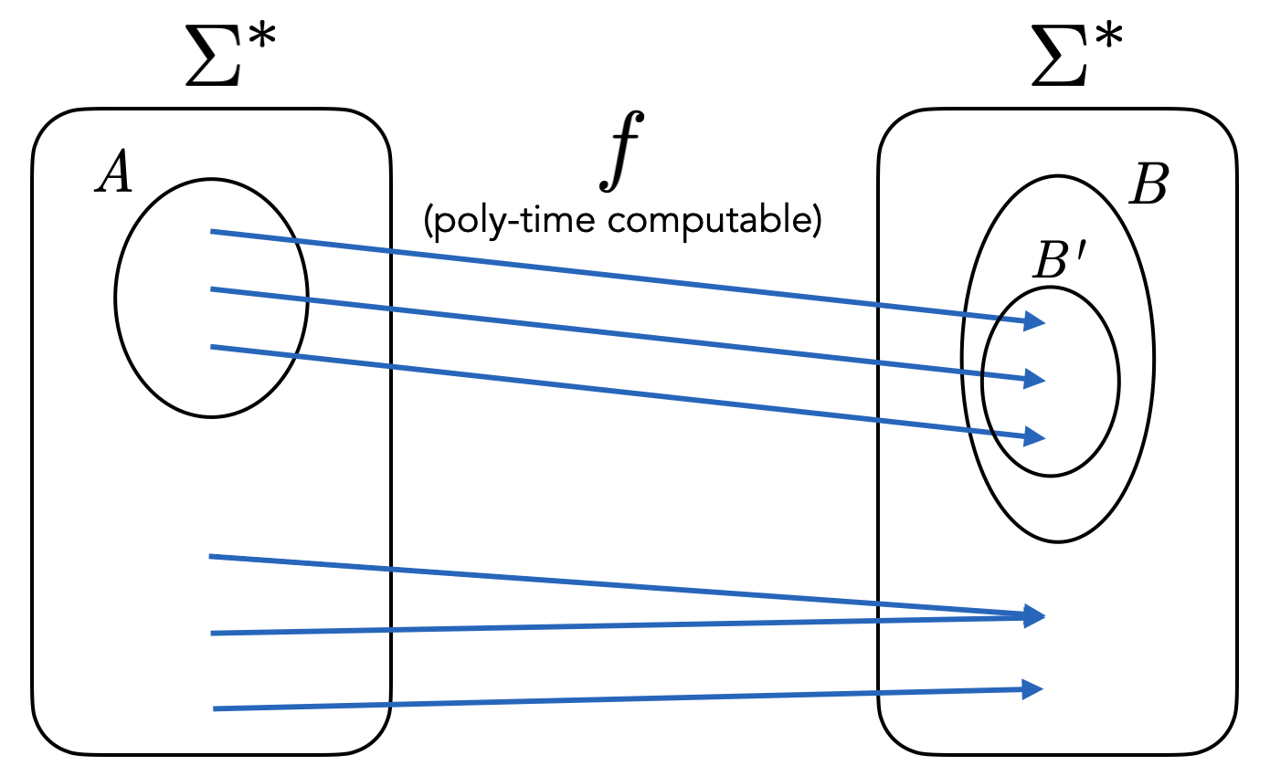
So typically, the transformation does not cover all the elements of $B$ , but only a subset $B' \subset B$ . This means that the Karp reduction not only establishes that $B$ is $\mathsf{NP}$ -hard, but also that $B'$ is $\mathsf{NP}$ -hard.

Theorem (IS is

\mathsf{NP}

-complete)

$\text{IS}$ is $\mathsf{NP}$ -complete.

Note (Overview of reductions)

The collection of reductions that we have shown can be represented as follows:

Exercise (MSAT is

\mathsf{NP}

-complete)

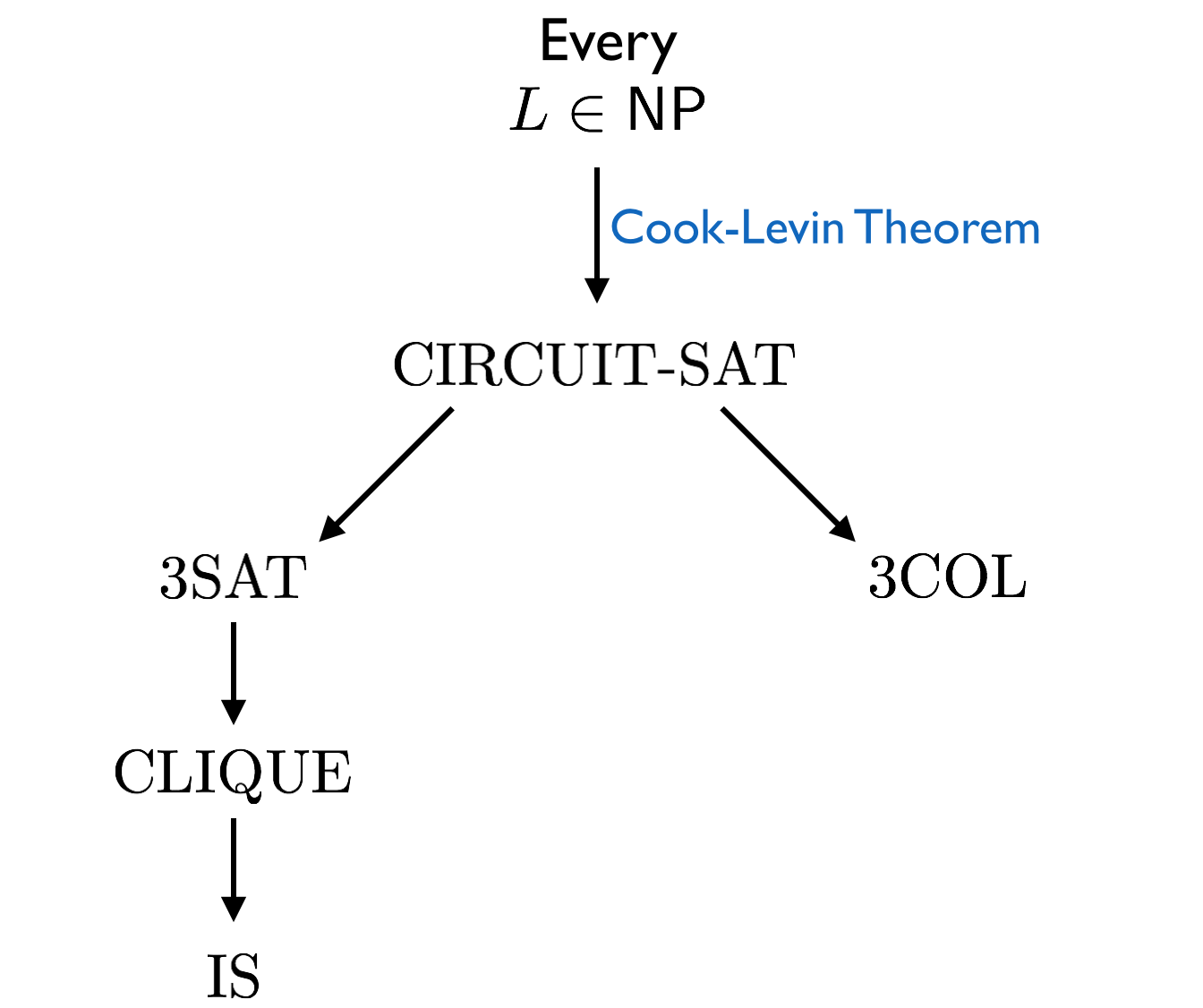
The MSAT problem is defined very similarly to SAT (for the definition of SAT, see Definition (Boolean satisfiability problem)). In SAT, we output True if and only if the input CNF formula has at least one satisfying truth assignment to the variables. In MSAT, we want to output True if and only if the input CNF formula has at least two distinct satisfying assignments.

Show that MSAT is $\mathsf{NP}$ -complete.

Exercise (BIN is

\mathsf{NP}

-complete)

In the PARTITION problem, we are given $n$ non-negative integers $a_1,a_2,\ldots, a_n$ , and we want to output True if and only if there is a way to partition the integers into two parts so that the sum of the two parts are equal. In other words, we want to output True if and only if there is a set $S \subseteq \{1,2,\ldots, n\}$ such that $\sum_{i \in S} a_i = \sum_{j \in \{1,\ldots,n\} \backslash S} a_j$ .

In the BIN problem we are given a set of n items with non-negative sizes $s_1, s_2, \ldots , s_n \in \mathbb N$ (not necessarily distinct), a capacity $C \geq 0$ (not necessarily an integer), and an integer $k \in \mathbb N$ . We want to output True if and only if the items can be placed into at most $k$ bins such that the total size of items in each bin does not exceed the capacity $C$ .

Show that BIN is $\mathsf{NP}$ -complete assuming PARTITION is $\mathsf{NP}$ -hard.

3. Check Your Understanding

Problem

Informally, at a high-level, what does it mean for a language to be in $\mathsf{NP}$ ?
Give an example of a language in $\mathsf{NP}$ and at a high level explain why it is in $\mathsf{NP}$ .
What are the things you need to show in order to formally argue that a language $L$ is in $\mathsf{NP}$ ?
Why is the complexity class $\mathsf{NP}$ named “Non-deterministic polynomial time”?
True or false: Every language in $\mathsf{NP}$ is decidable.
True or false: Any finite language is in $\mathsf{NP}$ .
True or false: $\{0,1\}^* \in \mathsf{NP}$ .
True or false: $\{0^k1^k : k \in \mathbb N\} \in \mathsf{NP}$ .
Explain why $\mathsf{P}$ is contained in $\mathsf{NP}$ .
True or false: If there is a polynomial-time algorithm for 3COL, then $\mathsf{P}= \mathsf{NP}$ .
True or false: HALTS is $\mathsf{NP}$ -complete.
Explain why $\mathsf{NP}$ is contained in $\mathsf{EXP}$ .
State the Cook-Levin Theorem and explain its significance.
Let $L \subseteq \Sigma^*$ , and define its complement $\overline{L} = \{w \in \Sigma^* : w \not\in L\}$ . Define $\textsf{coNP} = \{L \subseteq \Sigma^* : \overline{L} \in \mathsf{NP}\}$ . True or false: If $\textsf{coNP} \neq \mathsf{NP}$ , then $\mathsf{P}\neq \mathsf{NP}$ .
True or false: If every language in $\mathsf{NP}$ is $\mathsf{NP}$ -complete (under Cook reductions) then $\mathsf{P}= \mathsf{NP}$ .
True or false: If $\mathsf{P}= \mathsf{NP}$ then every language in $\mathsf{NP}$ is $\mathsf{NP}$ -complete (under Cook reductions).
True or false: For any two $\mathsf{NP}$ -complete languages $A$ and $B$ , there is a Cook reduction from $A$ to $B$ .
True or false: Let $L = \{0^k1^k : k \in \mathbb N\}$ . There is a Karp reduction from $L$ to 3COL.
Assume $\mathsf{P}\neq \mathsf{NP}$ . Does 2COL Karp reduce to 3COL?
Assume $\mathsf{P}\neq \mathsf{NP}$ . Does 3COL Karp reduce to 2COL?

4. High-Order Bits

Important Note

Non-deterministic polynomial time is one of the most important definitions in the course. The formal definition is not easy to understand at first since it has several layers. Take your time to really digest it, and be careful with the order of quantifiers.
When we ask you to show that a language is in $\mathsf{NP}$ , we expect you to use the formal definition of $\mathsf{NP}$ . Your proofs should resemble the proofs presented in this chapter.
It is guaranteed that you will see an $\mathsf{NP}$ -completeness proof in the homework and exam. In this course, your reductions establishing $\mathsf{NP}$ -hardness must be Karp reductions. This chapter contains various such arguments, and we expect your own arguments to follow a similar structure. As usual, do not fall in the trap of memorizing templates. Focus on understanding why the proofs are structured the way they are.

Probability Theory Basics

1. Basic Definitions and Properties

Definition (Finite probability space, sample space, probability distribution)

A finite probability space is a tuple $(\Omega, \Pr)$ , where

$\Omega$ is a non-empty finite set called the sample space;
$\Pr : \Omega \to [0,1]$ is a function, called the probability distribution, with the property that $\sum_{\ell \in \Omega} \Pr[\ell] = 1$ .

The elements of $\Omega$ are called outcomes or samples. If $\Pr[\ell] = p$ , then we say that the probability of outcome $\ell$ is $p$ .

Note (Modeling randomness)

The abstract definition above of a finite probability space helps us to mathematically model and reason about situations involving randomness and uncertainties (these situations are often called “random experiments” or just “experiments”). For example, consider the experiment of flipping a single coin. We model this as follows. We let $\Omega = \{\text{Heads}, \text{Tails}\}$ and we define function $\Pr$ such that $\Pr[\text{Heads}] = 1/2$ and $\Pr[\text{Tails}] = 1/2$ . This corresponds to our intuitive understanding that the probability of seeing the outcome Heads is $1/2$ and the probability of seeing the outcome Tails is also $1/2$ .

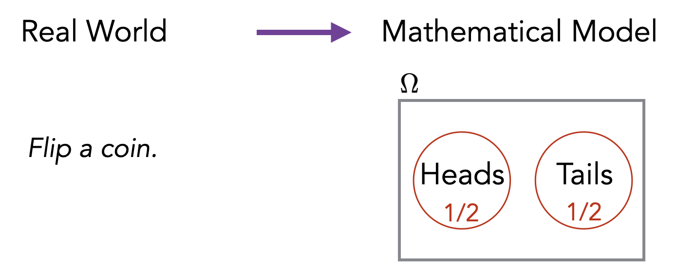
If we flip two coins, the sample space would look as follows (H represents “Heads” and T represents “Tails”).

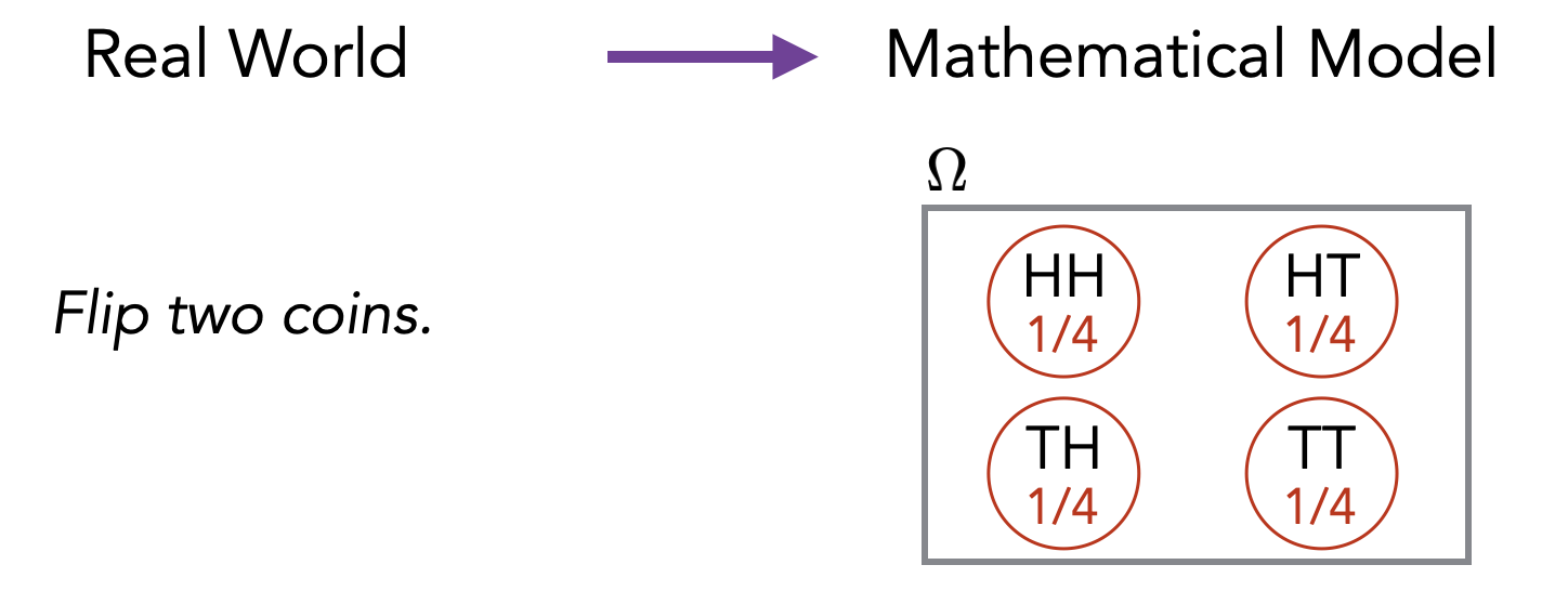
One can visualize the probability space as a circle or pie with area 1. Each outcome gets a slice of the pie proportional to its probability.

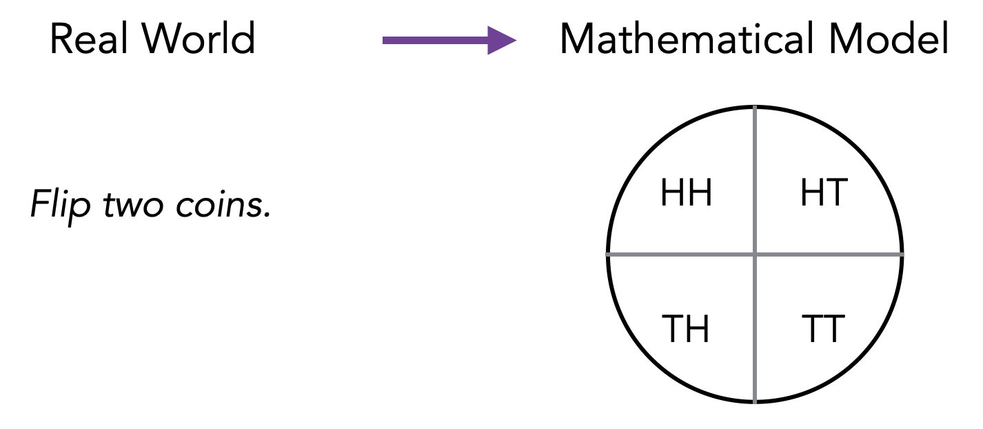
Note (Restriction to finite sample spaces)

In this course, we’ll usually restrict ourselves to finite sample spaces. In cases where we need a countably infinite $\Omega$ , the above definition will generalize naturally.

Exercise (Probability space modeling)

How would you model a roll of a single $6$ -sided die using Definition (Finite probability space, sample space, probability distribution)? How about a roll of two dice? How about a roll of a die and a coin toss together?

Note (Modeling through randomized code)

Sometimes, the modeling of a real-world random experiment as a probability space can be non-trivial or tricky. It helps a lot to have a step in between where you first go from the real-world experiment to computer code/algorithm (that makes calls to random number generators), and then you define your probability space based on the computer code. In this course, we allow our programs to have access to the functions $\text{Bernoulli}(p)$ and $\text{RandInt}(n)$ . The function $\text{Bernoulli}(p)$ takes a number $0 \leq p \leq 1$ as input and returns $1$ with probability $p$ and $0$ with probability $1-p$ . The function $\text{RandInt}(n)$ takes a positive integer $n$ as input and returns a random integer from $1$ to $n$ (i.e., every number from $1$ to $n$ has probability $1/n$ ). Here is a very simple example of going from a real-world experiment to computer code. The experiment is as follows. You flip a fair coin. If it’s heads, you roll a $3$ -sided die. If it is tails, you roll a $4$ -sided die. This experiment can be represented as:

    flip = Bernoulli(1/2)
    if flip == 0:
        die = RandInt(3)
    else:
        die = RandInt(4)

If we were to ask “What is the probability that you roll a 3 or higher?”, this would correspond to asking what is the probability that after the above code is executed, the variable named die stores a value that is 3 or higher.

One advantage of modeling with randomized code is that if there is any ambiguity in the description of the random (real-world) experiment, then it would/should be resolved in this step of creating the randomized code.

The second advantage is that it allows you to easily imagine a probability tree associated with the randomized code. The probability tree gives you clear picture on what the sample space is and how to compute the probabilities of the outcomes. The probability tree corresponding to the above code is as follows.

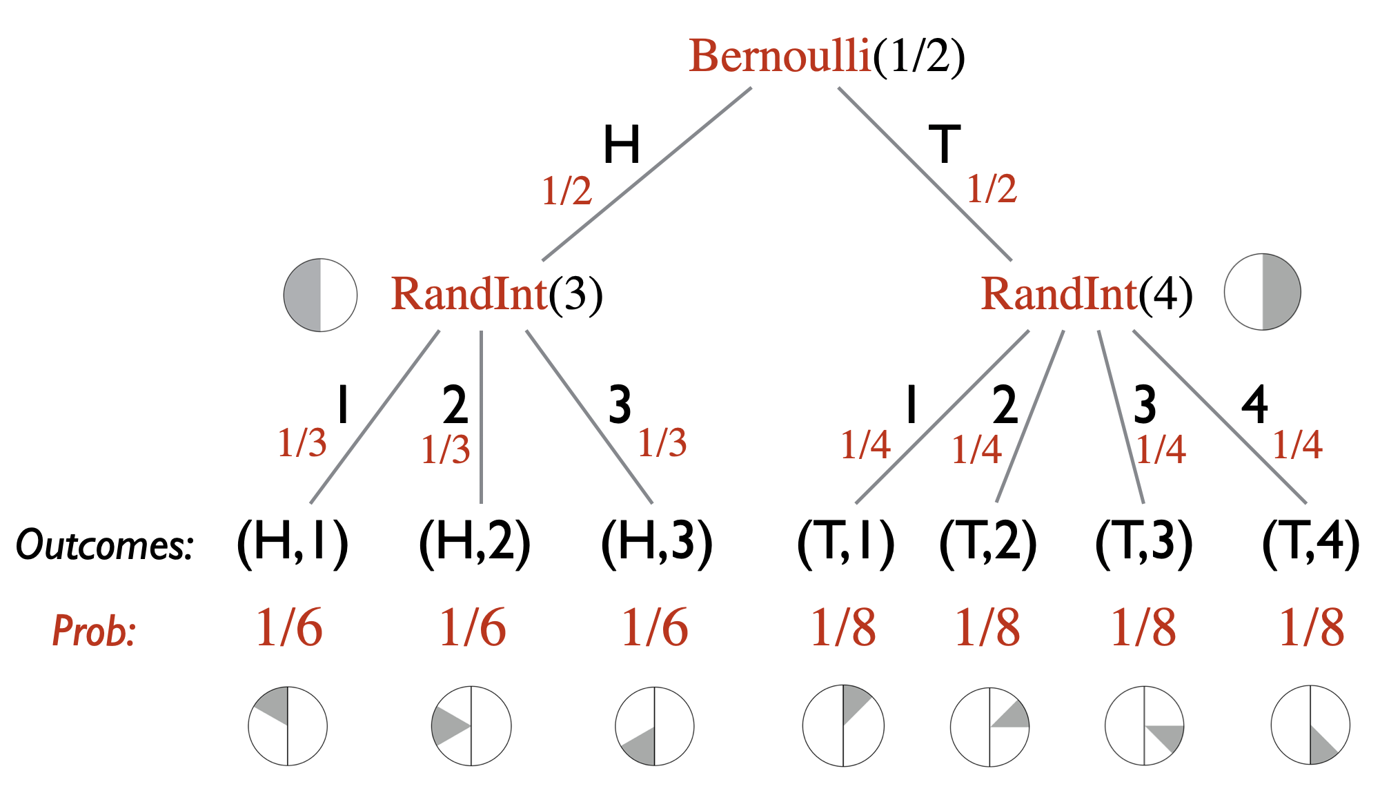
This simple example may not illustrate the usefulness of having a computer code representation of the random experiment, but one can appreciate its value with more sophisticated examples and we do encourage you to think of random experiments as computer code: $\text{real-world experiment} \longrightarrow \text{computer code / probability tree} \longrightarrow \text{probability space } (\Omega, \Pr).$

Definition (Uniform distribution)

If a probability distribution $\Pr : \Omega \to [0,1]$ is such that $\Pr[\ell] = 1/|\Omega|$ for all $\ell \in \Omega$ , then we call it a uniform distribution.

Definition (Event)

Let $(\Omega, \Pr)$ be a probability space. Any subset of outcomes $E \subseteq \Omega$ is called an event. We extend the $\Pr[\cdot]$ notation and write $\Pr[E]$ to denote $\sum_{\ell \in E} \Pr[\ell]$ . Using this notation, $\Pr[\varnothing] = 0$ and $\Pr[\Omega] = 1$ . We use the notation $\overline{E}$ to denote the event $\Omega \backslash E$ .

Exercise (Practice with events)

Suppose we roll two $6$ -sided dice. How many events are there? Write down the event corresponding to “we roll a double” and determine its probability.
Suppose we roll a $3$ -sided die and see the number $d$ . We then roll a $d$ -sided die. How many different events are there? Write down the event corresponding to “the second roll is a $2$ ” and determine its probability.

Exercise (Basic facts about probability)

Let $A$ and $B$ be two events. Prove the following.

If $A \subseteq B$ , then $\Pr[A] \leq \Pr[B]$ .
$\Pr[\overline{A}] = 1 - \Pr[A]$ .
$\Pr[A \cup B] = \Pr[A] + \Pr[B] - \Pr[A \cap B]$ .

Definition (Disjoint events)

We say that two events $A$ and $B$ are disjoint events if $A \cap B = \varnothing$ .

Exercise (Union bound)

Let $A_1,A_2,\ldots,A_n$ be events. Then $\Pr[A_1 \cup A_2 \cup \cdots \cup A_n] \leq \Pr[A_1] + \Pr[A_2] + \cdots + \Pr[A_n].$ We get equality if and only if the $A_i$ ’s are pairwise disjoint.

Definition (Conditional probability)

Let $E$ be an event with $\Pr[E] \neq 0$ . The conditional probability of outcome $\ell \in \Omega$ given $E$ , denoted $\Pr[\ell \; | \;E]$ , is defined as $\Pr[\ell \; | \;E] = \begin{cases} 0 &\text{if $\ell \not \in E$}\\ \frac{\Pr[\ell]}{\Pr[E]} &\text{if $\ell \in E$} \end{cases}$ For an event $A$ , the conditional probability of $A$ given $E$ , denoted $\Pr[A \; | \;E]$ , is defined as $\begin{aligned} \Pr[A \; | \;E] = \frac{\Pr[A \cap E]}{\Pr[E]}.\end{aligned}$

Note (Intuitive understanding of conditional probability)

Although it may not be immediately obvious, the above definition of conditional probability does correspond to our intuitive understanding of what conditional probability should represent. If we are told that event $E$ has already happened, then we know that the probability of any outcome outside of $E$ should be $0$ . Therefore, we can view the conditioning on event $E$ as a transformation of our probability space where we revise the probabilities (i.e., we revise the probability function $\Pr[\cdot]$ ). In particular, the original probability space $(\Omega, \Pr)$ gets transformed to $(\Omega, \Pr_E)$ , where $\Pr_E$ is such that for any $\ell \not \in E$ , we have $\Pr_E[\ell] = 0$ , and for any $\ell \in E$ , we have $\Pr_E[\ell] = \Pr[\ell] / \Pr[E]$ . The $1/\Pr[E]$ factor here is a necessary normalization factor that ensures the probabilities of all the outcomes sum to $1$ (which is required by Definition (Finite probability space, sample space, probability distribution)). Indeed, $\begin{aligned} \textstyle \sum_{\ell \in \Omega} \Pr_E[\ell] & = \textstyle \sum_{\ell \not \in E} \Pr_E[\ell] + \sum_{\ell \in E} \Pr_E[\ell] \\ & = \textstyle 0 + \sum_{\ell \in E} \Pr[\ell]/\Pr[E] \\ & = \textstyle \frac{1}{\Pr[E]} \sum_{\ell \in E} \Pr[\ell] \\ & = 1.\end{aligned}$ If we are interested in the event “ $A$ given $E$ ” (denoted by $A \; | \;E$ ) in the probability space $(\Omega, \Pr)$ , then we are interested in the event $A$ in the probability space $(\Omega, \Pr_E)$ . That is, $\Pr[A \; | \;E] = \Pr_E[A]$ . Therefore, $\textstyle \Pr[A \; | \;E] = \Pr_E[A] = \Pr_E[A \cap E] = \displaystyle \frac{\Pr[A \cap E]}{\Pr[E]},$ where the last equality holds by the definition of $\Pr_E[ \cdot ]$ . We have thus recovered the equality in Definition (Conditional probability).

Conditioning on event $E$ can also be viewed as redefining the sample space $\Omega$ to be $E$ , and then renormalizing the probabilities so that $\Pr[\Omega] = \Pr[E] = 1$ .

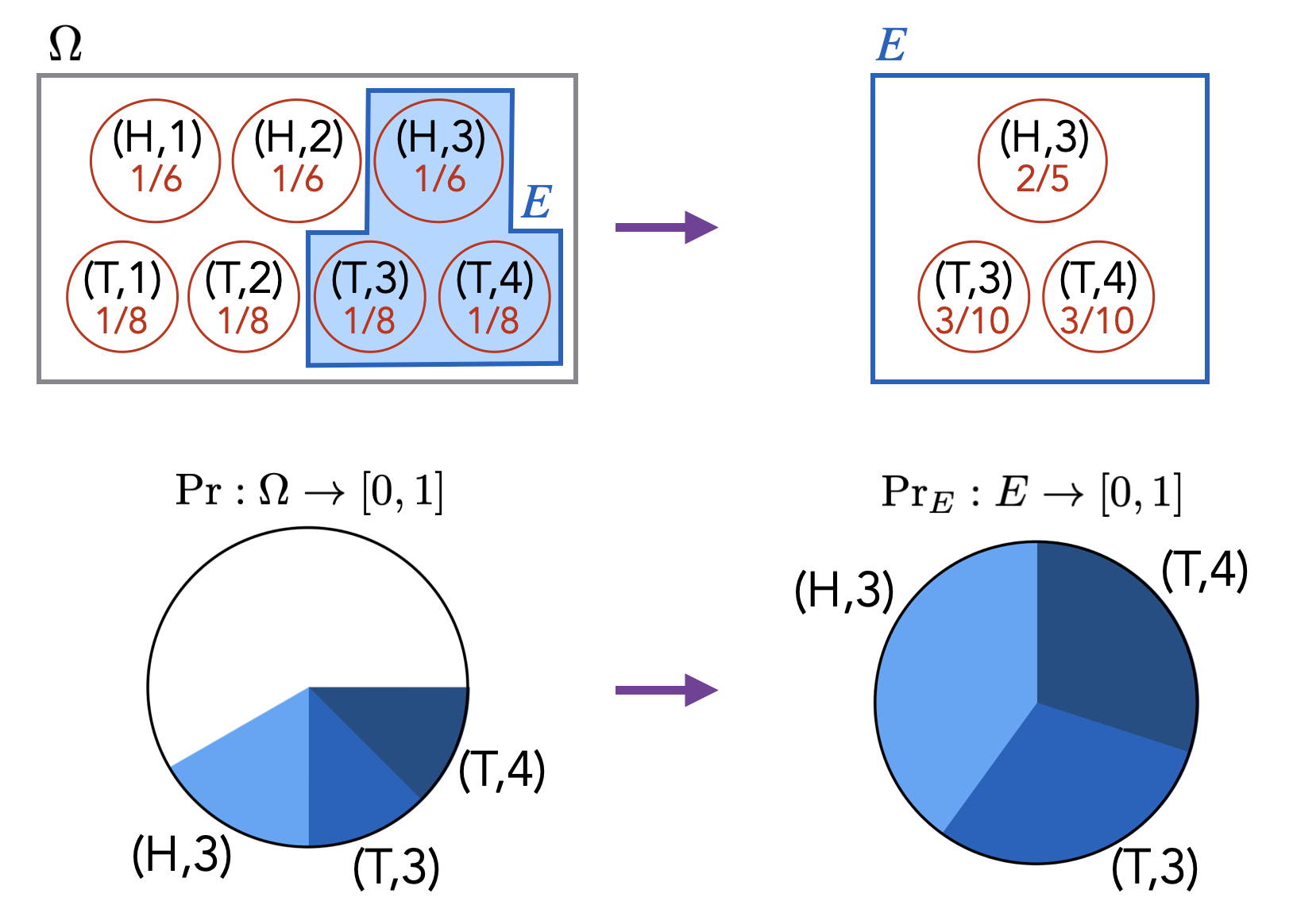
Exercise (Conditional probability practice)

Suppose we roll a $3$ -sided die and see the number $d$ . We then roll a $d$ -sided die. We are interested in the probability that the first roll was a $1$ given that the second roll was a $1$ . First express this probability using the notation of conditional probability and then determine what the probability is.

Proposition (Chain rule)

Let $n \geq 2$ and let $A_1,A_2,\ldots,A_n$ be events. Then $\begin{aligned} & \Pr[A_1 \cap \cdots \cap A_n] = \\ & \qquad \Pr[A_1] \cdot \Pr[A_2 \; | \;A_1] \cdot \Pr[A_3 \; | \;A_1 \cap A_2] \cdots \Pr[A_n \; | \;A_1 \cap A_2 \cap \cdots \cap A_{n-1}].\end{aligned}$

Exercise (Practice with chain rule)

Suppose there are 100 students in 15-251 and 5 of the students are Andrew Yang supporters. We pick 3 students from class uniformly at random. Calculate the probability that none of them are Andrew Yang supporters using Proposition (Chain rule).

Definition (Independent events)

Let $A$ and $B$ be two events. We say that $A$ and $B$ are independent events if $\Pr[A \cap B] = \Pr[A]\cdot \Pr[B]$ . Note that if $\Pr[B] \neq 0$ , then this is equivalent to $\Pr[A \; | \;B] = \Pr[A]$ . If $\Pr[A] \neq 0$ , it is also equivalent to $\Pr[B \; | \;A] = \Pr[B]$ .
Let $A_1, A_2,\ldots, A_n$ be events. We say that $A_1,\ldots,A_n$ are independent if for any subset $S \subseteq \{1,2,\ldots,n\}$ , $\Pr\left[\bigcap_{i \in S} A_i\right] = \prod_{i\in S} \Pr[A_i].$

Note (Defining independence through computer code)

Above we have given the definition of independent events as presented in 100% of the textbooks on probability theory. Yet, there is something deeply unsatisfying about this definition. In many situations people want to compute a probability of the form $\Pr[A \cap B]$ , and if possible (if they are independent), would like to use the equality $\Pr[A \cap B] = \Pr[A] \Pr[B]$ to simplify the calculation. In order to do this, they will informally argue that events $A$ and $B$ are independent in the intuitive sense of the word. For example, they argue that if $B$ happens, then this doesn’t affect the probability of $A$ happening (this argument is not done by calculation, but by informal argument). Then using this, they justify using the equality $\Pr[A \cap B] = \Pr[A] \Pr[B]$ in their calculations. So really, secretly, people are not using Definition (Independent events) but some other non-formal intuitive definition of independence, and then concluding what the formal definition says, which is $\Pr[A \cap B] = \Pr[A] \Pr[B]$ .

To be a bit more explicit, recall that the approach to answering probability related questions is to go from a real-world experiment we want to analyze to a formal probability space model: $\text{real-world experiment} \longrightarrow \text{probability space } (\Omega, \Pr).$ People often argue the independence of events $A$ and $B$ on the left-hand-side in order to use $\Pr[A \cap B] = \Pr[A] \Pr[B]$ on the right-hand-side. The left-hand-side, however, is not really a formal setting and may have ambiguities. And why does our intuitive notion of independence allow us to conclude $\Pr[A \cap B] = \Pr[A] \Pr[B]$ ? In these situations, it helps to add the “computer code” step in between: $\text{real-world experiment} \longrightarrow \text{computer code} \longrightarrow \text{probability space } (\Omega, \Pr).$ Computer code has no ambiguities and we can give a formal definition of independence using it. Suppose you have a randomized code modeling the real-world experiment, and suppose that you can divide the code into two separate parts. Suppose $A$ is an event that depends only on the first part of the code, and $B$ is an event that depends only on the second part of the code. If you can prove that the two parts of the code cannot affect each other, then we say that $A$ and $B$ are independent. When $A$ and $B$ are independent in this sense, then one can verify that indeed the equality $\Pr[A \cap B] = \Pr[A] \Pr[B]$ holds.

Proposition (Law of total probability)

Let $A_1,A_2,\ldots,A_n,B$ be events such that the $A_i$ ’s form a partition of the sample space $\Omega$ . Then $\Pr[B] = \Pr[B \cap A_1] + \Pr[B \cap A_2] + \cdots + \Pr[B \cap A_n].$ Equivalently, $\Pr[B] = \Pr[A_1]\cdot \Pr[B \; | \;A_1] + \Pr[A_2]\cdot \Pr[B \; | \;A_2] + \cdots + \Pr[A_n]\cdot \Pr[B \; | \;A_n].$

Exercise (Proof of the law of total probability)

Prove the above proposition.

Exercise (Practice with the law of total probability)

There are 2 bins. Bin 1 contains 6 red balls and 4 blue balls. Bin 2 contains 3 red balls and 7 blue balls. We choose a bin uniformly at random, and then choose one of the balls in that bin uniformly at random. Calculate the probability that the chosen ball is red using Proposition (Law of total probability).

2. Random Variables Basics

Definition (Random variable)

A random variable is a function $\mathbf{X} : \Omega \to \mathbb R$ , where $\Omega$ is a sample space.

Note (Random variable intuition)

Note that a random variable is just a labeling of the elements in $\Omega$ with some real numbers. One can think of this as a transformation of the original sample space into one that contains only numbers. For example, suppose the original sample space corresponds to flipping two coins. Then we can define a random variable $\mathbf{X}$ which maps an outcome in the sample space to the number of tails in the outcome. Since we are only flipping two coins, the possible outputs of $\mathbf{X}$ are $0$ , $1$ , and $2$ .

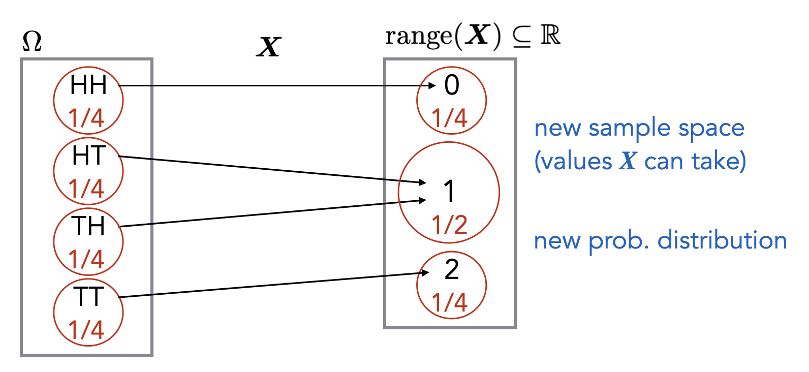
This kind of transformation is often desirable. For example, the transformation allows us to take a weighted average of the elements in the new sample space, where the weights correspond to the probabilities of the elements (if the distribution is uniform, the weighted average is just the regular average). This is called the expectation of the random variable and is formally defined below in Definition (Expected value of a random variable). Without this transformation into real numbers, the concept of an “expected value” (i.e. averaging) would not be possible to define.

Remark (Range of a random variable)

Almost always, the random variables we consider in this course will have a range that is a subset of $\mathbb N$ .

Definition (Common events through a random variable)

Let $\mathbf{X}$ be a random variable and $x \in \mathbb R$ be some real value. We use $\begin{aligned} \mathbf{X}=x & \quad \text{ to denote the event $\{\ell \in \Omega : \mathbf{X}(\ell) = x \}$},\\ \mathbf{X} \leq x & \quad \text{ to denote the event $\{\ell \in \Omega : \mathbf{X}(\ell) \leq x \}$},\\ \mathbf{X} \geq x & \quad \text{ to denote the event $\{\ell \in \Omega : \mathbf{X}(\ell) \geq x \}$},\\ \mathbf{X} < x & \quad \text{ to denote the event $\{\ell \in \Omega : \mathbf{X}(\ell) < x \}$},\\ \mathbf{X} > x & \quad \text{ to denote the event $\{\ell \in \Omega : \mathbf{X}(\ell) > x \}$}.\end{aligned}$ For example, $\Pr[\mathbf{X}=x]$ denotes $\Pr[\{\ell \in \Omega : \mathbf{X}(\ell) = x\}]$ . More generally, for $S \subseteq \mathbb R$ , we use $\begin{aligned} \mathbf{X} \in S & \quad \text{ to denote the event $\{\ell \in \Omega : \mathbf{X}(\ell) \in S \}$}.\end{aligned}$

Exercise (Practice with random variables)

Suppose we roll two $6$ -sided dice. Let $\mathbf{X}$ be the random variable that denotes the sum of the numbers we see. Explicitly write down the input-output pairs for the function $\mathbf{X}$ . Calculate $\Pr[\mathbf{X} \geq 7]$ .

Note (Random variables and randomized code)

Using the randomized code and probability tree point of view, we can simply define a random variable as a numerical variable in some randomized code (more accurately, the variable’s value at the end of the execution of the code). For example, consider the following randomized code.

    S = RandInt(6) + RandInt(6)
    if S == 12:
        I = 1
    else:
        I = 0

Here we have two random variables corresponding to the variables in the code, $\mathbf{S}$ and $\mathbf{I}$ . From the probability tree picture, we can see how these two random variables can be viewed as functions from the sample space (the set of leaves) to $\mathbb R$ since they map each leaf/outcome to some numerical value.

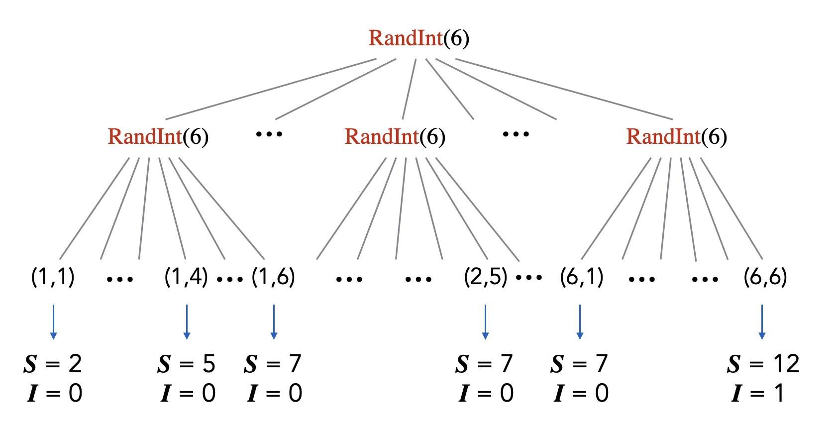
Note (Forgetting the original sample space)

Given some probability space $(\Omega, \Pr)$ and a random variable $\mathbf{X} : \Omega \to \mathbb R$ , we often forget about the original sample space and consider the sample space to be the range of $\mathbf{X}$ , $\text{range}(\mathbf{X}) = \{\mathbf{X}(\ell): \ell \in \Omega\}$ .

Definition (Probability mass function (PMF))

Let $\mathbf{X} : \Omega \to \mathbb R$ be a random variable. The probability mass function (PMF) of $\mathbf{X}$ is a function $p_{\mathbf{X}} : \mathbb R\to [0,1]$ such that for any $x \in \mathbb R$ , $p_{\mathbf{X}}(x) = \Pr[\mathbf{X} = x]$ .

Note (Defining a random variable through PMF)

Related to the previous remark, we sometimes “define” a random variable by just specifying its probability mass function. In particular, we make no mention of the underlying sample space.

Definition (Expected value of a random variable)

Let $\mathbf{X}$ be a random variable. The expected value of $\mathbf{X}$ , denoted $\mathbb E[\mathbf{X}]$ , is defined as follows: $\mathbb E[\mathbf{X}] = \sum_{\ell \in \Omega} \Pr[\ell]\cdot \mathbf{X}(\ell).$ Equivalently, $\mathbb E[\mathbf{X}] = \sum_{x \in \text{range}(\mathbf{X})} \Pr[\mathbf{X}=x]\cdot x,$ where $\text{range}(\mathbf{X}) = \{\mathbf{X}(\ell): \ell \in \Omega\}$ .

Exercise (Equivalence of expected value definitions)

Prove that the above two expressions for $\mathbb E[\mathbf{X}]$ are equivalent.

Exercise (Practice with expected value)

Suppose we roll two $6$ -sided dice. Let $\mathbf{X}$ be the random variable that denotes the sum of the numbers we see. Calculate $\mathbb E[\mathbf{X}]$ .

Note (Arithmetic operations on random variables)

Fix some sample space $\Omega$ and consider random variables on this sample space. Since random variables are functions from $\Omega$ to $\mathbb R$ , arithmetic operations on random variables are arithmetic operations on functions, and these arithmetic operations produce a new random variable. For example, if $\mathbf{X}$ and $\mathbf{Y}$ are random variables, then an expression like $\mathbf{X} + 2\mathbf{X}\mathbf{Y}$ denotes a new random variable, because it is also a function from $\Omega$ to $\mathbb R$ .

Proposition (Linearity of expectation)

Let $\mathbf{X}$ and $\mathbf{Y}$ be two random variables, and let $c_1,c_2 \in \mathbb R$ be some constants. Then $\mathbb E[c_1\mathbf{X}+c_2\mathbf{Y}] = c_1\mathbb E[\mathbf{X}] + c_2\mathbb E[\mathbf{Y}].$

Corollary (Linearity of expectation 2)

Let $\mathbf{X}_1,\mathbf{X}_2,\ldots,\mathbf{X}_n$ be random variables, and $c_1,c_2,\ldots,c_n \in \mathbb R$ be some constants. Then $\mathbb E[c_1\mathbf{X}_1 + c_2\mathbf{X}_2 + \cdots + c_n\mathbf{X}_n] = c_1\mathbb E[\mathbf{X}_1] + c_2\mathbb E[\mathbf{X}_2] + \cdots + c_n\mathbb E[\mathbf{X}_n].$ In particular, when all the $c_i$ ’s are 1, we get $\mathbb E[\mathbf{X}_1 + \mathbf{X}_2 + \cdots + \mathbf{X}_n] = \mathbb E[\mathbf{X}_1] + \mathbb E[\mathbf{X}_2] + \cdots + \mathbb E[\mathbf{X}_n].$

Exercise (Practice with linearity of expectation)

Suppose we roll three $10$ -sided dice. Let $\mathbf{X}$ be the sum of the three values we see. Calculate $\mathbb E[\mathbf{X}]$ .

Exercise (Expectation of the product of random variables)

Define two random variables $\mathbf{X}$ and $\mathbf{Y}$ such that $\mathbb E[\mathbf{X}\mathbf{Y}] \neq \mathbb E[\mathbf{X}] \mathbb E[\mathbf{Y}]$ .

Definition (Indicator random variable)

Let $E \subseteq \Omega$ be some event. The indicator random variable with respect to $E$ is denoted by $\mathbf{I}_E$ and is defined as $\mathbf{I}_E(\ell) = \begin{cases} 1 & \quad \text{if $\ell \in E$,}\\ 0 & \quad \text{otherwise.}\\ \end{cases}$

Proposition (Expectation of an indicator random variable)

Let $E$ be an event. Then $\mathbb E[\mathbf{I}_E] = \Pr[E]$ .

Important Note (Combining linearity of expectation and indicators)

Suppose that you are interested in computing $\mathbb E[\mathbf{X}]$ for some random variable $\mathbf{X}$ . If you can write $\mathbf{X}$ as a sum of indicator random variables, i.e., if $\mathbf{X} = \sum_j \mathbf{I}_{E_j}$ where $\mathbf{I}_{E_j}$ are indicator random variables, then by linearity of expectation, $\mathbb E[\mathbf{X}] = \mathbb E\left[\sum_j \mathbf{I}_{E_j}\right] = \sum_j \mathbb E[\mathbf{I}_{E_j}].$ Furthermore, by Proposition (Expectation of an indicator random variable), we know $\mathbb E[\mathbf{I}_{E_j}] = \Pr[E_j]$ . Therefore $\mathbb E[\mathbf{X}] = \sum_j \Pr[E_j]$ . This often provides an extremely convenient way of computing $\mathbb E[\mathbf{X}]$ . This combination of indicator random variables together with linearity expectation is one of the most useful tricks in probability theory!

Exercise (Practice with linearity of expectation and indicators)

There are $n$ balls and $n$ bins. For each ball, you pick one of the bins uniformly at random and drop the ball in that bin. What is the expected number of balls in bin 1? What is the expected number of empty bins?
Suppose you randomly color the vertices of the complete graph on $n$ vertices one of $k$ colors. What is the expected number of paths of length $c$ (where we assume $c \geq 3$ ) such that no two adjacent vertices on the path have the same color?

Theorem (Markov’s inequality)

Let $\mathbf{X}$ be a non-negative random variable. Then for any $c > 0$ , $\Pr[\mathbf{X} \geq c \cdot \mathbb E[\mathbf{X}]] \leq \frac{1}{c}.$ Or equivalently, $\Pr[\mathbf{X} \geq c] \leq \frac{\mathbb E[\mathbf{X}]}{c}.$

Exercise (Practice with Markov’s inequality)

During the Spring 2022 semester, the 15-251 TAs decide to strike because they are not happy with the lack of free food in grading sessions. Without the TA support, the performance of the students in the class drop dramatically. The class average on the first midterm exam is 15%. Using Markov’s Inequality, give an upper bound on the fraction of the class that got an A (i.e., at least a 90%) in the exam.

3. Three Popular Random Variables

Definition (Bernoulli random variable)

Let $0 < p < 1$ be some parameter. If $\mathbf{X}$ is a random variable with probability mass function $p_{\mathbf{X}}(1) = p$ and $p_{\mathbf{X}}(0) = 1-p$ , then we say that $\mathbf{X}$ has a Bernoulli distribution with parameter $p$ (we also say that $\mathbf{X}$ is a Bernoulli random variable). We write $\mathbf{X} \sim \text{Bernoulli}(p)$ to denote this. The parameter $p$ is often called the success probability.

Note (What does a Bernoulli random variable represent?)

A Bernoulli random variable $\text{Bernoulli}(p)$ captures a random experiment where we toss a $p$ -biased coin where the probability of heads is $p$ (and we assign this the numerical outcome of $1$ ) and the probability of tails is $1-p$ (and we assign this the numerical outcome of $0$ ).

Note (Expectation of Bernoulli random variable)

Note that $\mathbb E[\mathbf{X}] = 0 \cdot p_{\mathbf{X}}(0) + 1 \cdot p_{\mathbf{X}}(1) = p_{\mathbf{X}}(1) = p$ .

Definition (Binomial random variable)

Let $\mathbf{X} = \mathbf{X}_1 + \mathbf{X}_2 + \cdots + \mathbf{X}_n$ , where the $\mathbf{X}_i$ ’s are independent and for all $i$ , $\mathbf{X}_i \sim \text{Bernoulli}(p)$ . Then we say that $\mathbf{X}$ has a binomial distribution with parameters $n$ and $p$ (we also say that $\mathbf{X}$ is a binomial random variable). We write $\mathbf{X} \sim \text{Bin}(n,p)$ to denote this.

Note (What does a Binomial random variable represent?)

A Binomial random variable $\mathbf{X} \sim \text{Bin}(n,p)$ captures a random experiment where we toss a $p$ -biased coin $n$ times. We are interested in the probability of seeing $k$ heads among those $n$ coin tosses, where $k$ ranges over $\{0,1,2,\ldots, n\} = \text{range}(\mathbf{X})$ .

Note (Bernoulli is a special case of Binomial)

Note that we can view a Bernoulli random variable as a special kind of a binomial random variable where $n = 1$ .

Exercise (Expectation of a Binomial random variable)

Let $\mathbf{X}$ be a random variable with $\mathbf{X} \sim \text{Bin}(n,p)$ . Determine $\mathbb E[\mathbf{X}]$ (use linearity of expectation). Also determine $\mathbf{X}$ ’s probability mass function.

Exercise (Practice with Binomial random variable)

We toss a coin $5$ times. What is the probability that we see at least 4 heads? What is the expected number of heads?

Definition (Geometric random variable)

Let $\mathbf{X}$ be a random variable with probability mass function $p_{\mathbf{X}}$ such that for $n \in \{1,2,\ldots\}$ , $p_{\mathbf{X}}(n) = (1-p)^{n-1}p$ . Then we say that $\mathbf{X}$ has a geometric distribution with parameter $p$ (we also say that $\mathbf{X}$ is a geometric random variable). We write $\mathbf{X} \sim \text{Geometric}(p)$ to denote this.

Note (What does a Geometric random variable represent?)

A Geometric random variable $\text{Geometric}(p)$ captures a random experiment where we successively toss a $p$ -biased coin until we see heads for the first time, and we stop. We are interested in the probability of making $n$ coin tosses in total before we stop, where $n$ ranges over $\{1,2,\ldots\}$ .

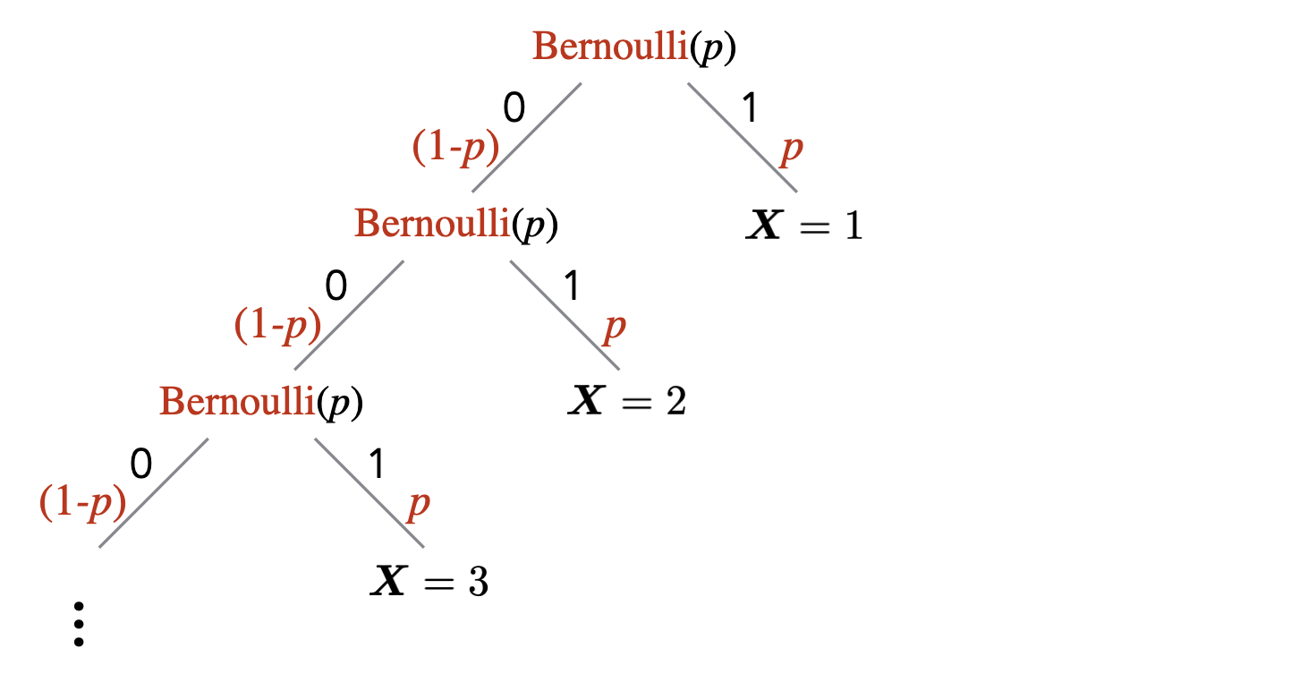
Exercise (PMF of a geometric random variable)

Let $\mathbf{X}$ be a geometric random variable. Verify that $\sum_{n = 1}^\infty p_{\mathbf{X}}(n) = 1$ .

Exercise (Practice with geometric random variable)

Suppose we repeatedly flip a coin until we see a heads for the first time. What is the probability that we will flip the coin more than $5$ times?

Exercise (Expectation of a geometric random variable)

Let $\mathbf{X}$ be a random variable with $\mathbf{X} \sim \text{Geometric}(p)$ . Determine $\mathbb E[\mathbf{X}]$ .

Important Note (Some general tips)

Here are some general tips on probability calculations (this is not meant to be an exhaustive list).

If you are trying to upper bound $\Pr[A]$ , you can try to find $B$ with $A \subseteq B$ , and then bound $\Pr[B]$ . Note that if an event $A$ implies an event $B$ , then this means $A \subseteq B$ . Similarly, if you are trying to lower bound $\Pr[A]$ , you can try to find $B$ with $B \subseteq A$ , and then bound $\Pr[B]$ .
If you are trying to upper bound $\Pr[A]$ , you can try to lower bound $\Pr[\overline{A}]$ since $\Pr[A] = 1-\Pr[\overline{A}]$ . Similarly, if you are trying to lower bound $\Pr[A]$ , you can try to upper bound $\Pr[\overline{A}]$ .
In some situations, law of total probability can be very useful in calculating (or bounding) $\Pr[A]$ .
If you need to calculate $\Pr[A_1 \cap \cdots \cap A_n]$ , try the chain rule. If the events are independent, then this probability is equal to the product $\Pr[A_1] \cdots \Pr[A_n]$ . Note that the event “for all $i \in \{1,\ldots,n\}$ , $A_i$ ” is the same as $A_1 \cap \cdots \cap A_n$ .
If you need to upper bound $\Pr[A_1 \cup \cdots \cup A_n]$ , you can try to use the union bound. Note that the event “there exists an $i \in \{1,\ldots,n\}$ such that $A_i$ ” is the same as $A_1 \cup \cdots \cup A_n$ .
When trying to calculate $\mathbb E[\mathbf{X}]$ , try:
1. directly using the definition of expectation;
2. writing $\mathbf{X}$ as a sum of indicator random variables, and then using linearity of expectation.

4. Check Your Understanding

Problem

Describe what a probability tree is.
True or false: If two events $A$ and $B$ are independent, then their complements $\overline{A}$ and $\overline{B}$ are also independent. (The complement of an event $A$ is $\overline{A} = \Omega \backslash A$ .)
True or false: If events $A$ and $B$ are disjoint, then they are necessarily independent.
True or false: For all events $A,B$ , $\Pr[A \; | \;B] \le \Pr[A]$ .
True or false: For all events $A,B$ , $\Pr[\overline{A} \; | \;B] = 1- \Pr[A \; | \;B]$ .
True or false: For all events $A,B$ , $\Pr[A \; | \;\overline{B}] = 1 - \Pr[A \; | \;B]$ .
True or false: Assume that every time a baby is born, there is $1/2$ chance that the baby is a boy. A couple has two children. At least one of the children is a boy. The probability that both children are boys is $1/2$ .
What is the union bound?
What is the chain rule?
What is a random variable?
What is an indicator random variable?
What is the expectation of a random variable?
What is linearity of expectation?
When calculating the expectation of a random variable $\mathbf{X}$ , the strategy of writing $\mathbf{X}$ as a sum of indicator random variables and then using linearity of expectation is quite powerful. Explain how this strategy is carried out.
True or false: Let $\mathbf{X}$ be a random variable. If $\mathbb E[\mathbf{X}] = \mu$ , then $\Pr[\mathbf{X} = \mu] > 0$ .
True or false: For any random variable $\mathbf{X}$ , $\mathbb E[1/\mathbf{X}] = 1/\mathbb E[\mathbf{X}]$ .
True or false: For any random variable $\mathbf{X}$ , $\Pr[\mathbf{X} \geq \mathbb E[\mathbf{X}]] > 0$ .
True or false: For any non-negative random variable $\mathbf{X}$ , $\mathbb E[\mathbf{X}^2] \le \mathbb E[\mathbf{X}]^2$ .
True or false: For any random variable $\mathbf{X}$ , $\mathbb E[-\mathbf{X}^3] = - \mathbb E[\mathbf{X}^3]$ .
What is Markov’s inequality?
What is a Bernoulli random variable? Give one example.
What is the expectation of a Bernoulli random variable, and how do you derive it?
What is a Binomial random variable? Give one example.
What is the expectation of a Binomial random variable, and how do you derive it?
What is a Geometric random variable? Give one example.
What is the expectation of a Geometric random variable (justification not required)?
Let $\mathbf{X}$ and $\mathbf{Y}$ be random variables. Does the expression $\mathbb E[\mathbf{X} \; | \;\mathbf{Y}] = 0$ type-check?
Let $A$ be an event. Does the expression $\mathbb E[A] = 0$ type-check?

Randomized Algorithms

1. Monte Carlo and Las Vegas Algorithms

Definition (Monte Carlo algorithm)

Let $f : \Sigma^* \to \Sigma^*$ be a computational problem. Let $0 \leq \epsilon < 1$ be some parameter and $T :\mathbb N\to \mathbb N$ be some function. Suppose $A$ is a randomized algorithm such that

for all $x \in \Sigma^*$ , $\Pr[A(x) \neq f(x)] \leq \epsilon$ ;
for all $x \in \Sigma^*$ , $\Pr[\text{number of steps $A(x)$ takes is at most $T(|x|)$}] = 1$ .

(Note that the probabilities are over the random choices made by $A$ .) Then we say that $A$ is a $T(n)$ -time Monte Carlo algorithm that computes $f$ with $\epsilon$ probability of error.

Definition (Las Vegas algorithm)

Let $f : \Sigma^* \to \Sigma^*$ be a computational problem. Let $T :\mathbb N\to \mathbb N$ be some function. Suppose $A$ is a randomized algorithm such that

for all $x \in \Sigma^*$ , $\Pr[A(x) = f(x)] = 1$ , where the probability is over the random choices made by $A$ ;
for all $x \in \Sigma^*$ , $\mathbb{E}[\text{number of steps $A(x)$ takes}] \leq T(|x|)$ .

Then we say that $A$ is a $T(n)$ -time Las Vegas algorithm that computes $f$ .

Note (Randomized algorithms for optimization problems)

One can adapt the definitions above to define the notions of Monte Carlo algorithms and Las Vegas algorithms that compute decision problems (i.e. languages).

Exercise (Las Vegas to Monte Carlo)

Suppose you are given a Las Vegas algorithm $A$ that solves $f:\Sigma^* \to \Sigma^*$ in expected time $T(n)$ . Show that for any constant $\epsilon > 0$ , there is a Monte Carlo algorithm that solves $f$ in time $O(T(n))$ and error probability $\epsilon$ .

Exercise (Monte Carlo to Las Vegas)

Suppose you are given a Monte Carlo algorithm $A$ that runs in worst-case $T_1(n)$ time and solves $f:\Sigma^* \to \Sigma^*$ with success probability at least $p$ (i.e., for every input, the algorithm gives the correct answer with probability at least $p$ and takes at most $T_1(n)$ steps). Suppose it is possible to check in $T_2(n)$ time whether the output produced by $A$ is correct or not. Show how to convert $A$ into a Las Vegas algorithm that runs in expected time $O((T_1(n)+T_2(n))/p)$ .

2. Monte Carlo Algorithm for Min-Cut

Definition (Minimum cut problem)

In the minimum cut problem, the input is a connected undirected graph $G$ , and the output is a $2$ -coloring of the vertices, where each color is used at least once, such that the number of edges whose endpoints are colored differently is minimized (such edges are called cut edges). Equivalently, we want to output a non-empty subset $S \subsetneq V$ such that the number of edges between $S$ and $V\backslash S$ is minimized. Such a set $S$ is called a cut and the size of the cut is the number of edges between $S$ and $V\backslash S$ (note that the size of the cut is not the number of vertices). We denote this problem by $\text{MIN-CUT}$ .

Definition (Multi-graph)

A multi-graph $G=(V,E)$ is an undirected graph in which $E$ is allowed to be a multi-set. In other words, a multi-graph can have multiple edges between two vertices.

Definition (Contraction of two vertices in a graph)

Let $G=(V,E)$ be a multi-graph and let $u,v \in V$ be two vertices in the graph. Contraction of $u$ and $v$ produces a new multi-graph $G'=(V',E')$ . Informally, in $G'$ , we collapse/contract the vertices $u$ and $v$ into one vertex and preserve the edges between these two vertices and the other vertices in the graph. Formally, we remove the vertices $u$ and $v$ , and create a new vertex called $uv$ , i.e. $V' = V \backslash \{u,v\} \cup \{uv\}$ . The multi-set of edges $E'$ is defined as follows:

for each $\{u,w\} \in E$ with $w \neq v$ , we add $\{uv,w\}$ to $E'$ ;
for each $\{v,w\} \in E$ with $w \neq u$ , we add $\{uv,w\}$ to $E'$ ;
for each $\{w,w'\} \in E$ with $w,w' \not \in \{u,v\}$ , we add $\{w,w'\}$ to $E'$ .

Below is an example:

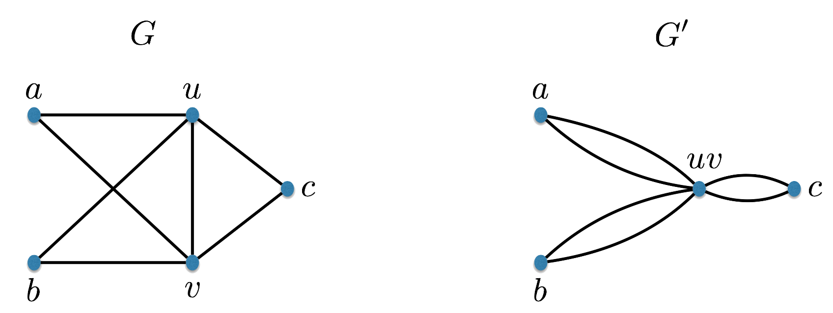
Theorem (Contraction algorithm for min cut)

There is a polynomial-time Monte-Carlo algorithm that solves the MIN-CUT problem with error probability at most $1/e^n$ , where $n$ is the number of vertices in the input graph.

Exercise (Boosting for one-sided error)

This question asks you to boost the success probability of a Monte Carlo algorithm computing a decision problem with one-sided error.

Let $f:\Sigma^* \to \{0,1\}$ be a decision problem, and let $A$ be a Monte Carlo algorithm for $f$ such that if $x$ is a YES instance, then $A$ always gives the correct answer, and if $x$ is a NO instance, then $A$ gives the correct answer with probability at least 1/2. Suppose $A$ runs in worst-case $O(T(n))$ time. Design a new Monte Carlo algorithm $A'$ for $f$ that runs in $O(nT(n))$ time and has error probability at most $1/2^n$ .

Exercise (Boosting for two-sided error)

This question asks you to boost the success probability of a Monte Carlo algorithm computing a decision problem with two-sided error.

Let $f:\Sigma^* \to \{0,1\}$ be a decision problem, and let $A$ be a Monte Carlo algorithm for $f$ with error probability $1/4$ , i.e., for all $x \in \Sigma^*$ , $\Pr[A(x) \neq f(x)] \leq 1/4$ . We want to boost the success probability to $1-1/2^n$ , and our strategy will be as follows. Given $x$ , run $A(x)$ $6n$ times (where $n = |x|$ ), and output the more common output bit among the $6n$ output bits (breaking ties arbitrarily). Show that the probability of outputting the wrong answer is at most $1/2^n$ .

Exercise (Maximum number of minimum cuts)

Using the analysis of the randomized minimum cut algorithm, show that a graph can have at most $n(n-1)/2$ distinct minimum cuts.

Exercise (Contracting two random vertices)

Suppose we modify the min-cut algorithm seen in lecture so that rather than picking an edge uniformly at random, we pick 2 vertices uniformly at random and contract them into a single vertex. True or False: The success probability of the algorithm (excluding the part that boosts the success probability) is $1/n^k$ for some constant $k$ , where $n$ is the number of vertices. Justify your answer.

3. Check Your Understanding

Problem

True or false: When analyzing a randomized algorithm, we assume that the input is chosen uniformly at random.
What is the difference between a Monte Carlo algorithm and a Las Vegas algorithm?
Describe the probability tree induced by a Monte Carlo algorithm on a given input.
Describe the probability tree induced by a Las Vegas algorithm on a given input.
Describe at a high level how to convert a Las Vegas algorithm into a Monte Carlo algorithm.
Describe at a high level how to covert a Monte Carlo algorithm into a Las Vegas algorithm.
In this chapter, we defined the MIN-CUT problem. In the MAX-CUT problem, given a graph $G=(V,E)$ , we want to output a subset $S \subseteq V$ such that the number of edges between $S$ and $V\backslash S$ is maximized. Suppose for every vertex $v \in V$ , we flip a fair coin and put the vertex in $S$ if the coin comes up heads. Show that the expected number of cut edges is $|E|/2$ .
Argue, using the result from previous question, why every graph with $|E|$ edges contains a cut of size at least $|E|/2$ .
Outline a general strategy for boosting the success probability of a Monte Carlo algorithm that computes a decision problem.
True or false: For any decision problem, there is a polynomial-time Monte Carlo algorithm that computes it with error probability equal to $1/2$ .
Suppose we have a Monte-Carlo algorithm for a decision problem with error probability equal to $1/2$ . Can we boost the success probability of this algorithm by repeated trials?
True or false: The cut output by the contraction algorithm is uniformly random among all possible cuts.
True or false: The size of a minimum cut in a graph is equal to the minimum degree of a vertex in the graph.
Give an example of a problem for which we have a polynomial-time randomized algorithm, but we do not know of a polynomial-time deterministic algorithm.

4. High-Order Bits

Important Note

As always, understanding the definitions is important. Make sure you are comfortable with the definitions of Monte Carlo and Las Vegas algorithms.
We require worst-case guarantees for randomized algorithms. In particular, in this course, we never consider a randomly chosen input.
One of the best ways to understand randomized algorithms is to have a clear understanding on how they induce a probability tree and what properties those probability trees have. We have emphasized this point of view in lecture even though it does not appear in this chapter.
It is important to know how to convert a Monte Carlo algorithm into a Las Vegas algorithm and vice versa.
The main example in this chapter is the analysis of the contraction algorithm for MIN-CUT. There are several interesting ideas in the analysis, and you should make note of those ideas/tricks. Especially the idea of boosting the success probability of a randomized algorithm via repeated trials is important.
One extremely useful trick that was highlighted in the previous chapter is the calculation of an expectation of a random variable by writing it as a sum of indicator random variables and using linearity of expectation (see Important Note (Combining linearity of expectation and indicators) and the exercise after it). This trick comes up a lot in the context of randomized algorithms. In particular, you will very likely be asked a question of the form “Give a randomized algorithm for problem X with the property that the expected number of Y is equal to Z.” As an example, see the analysis of the randomized algorithm for MAX-CUT problem covered in lecture.

Modular Arithmetic

1. Preliminary Definitions

Definition (

A

divides

B

)

Let $A, B \in \mathbb Z$ . We say that $A$ divides $B$ (or $A$ is a divisor of $B$ ), denoted $A | B$ , if there is a number $C \in \mathbb Z$ such that $B = AC$ .

Definition (Prime number)

Let $P \in \mathbb N$ . We say that $P$ is a prime number if $P \geq 2$ and the only divisors of $P$ are $1$ and $P$ .

Definition (Congruence modulo

N

)

Let $A, B$ and $N$ be positive integers. We denote by $A \bmod N$ the remainder you get when you divide $A$ by $N$ . Note that $A \bmod N \in \{0,1,2,\ldots,N-1\}$ . We say that $A$ and $B$ are congruent modulo $N$ , denoted $A \equiv_N B$ (or $A \equiv B \bmod N$ ), if $A \bmod N = B \bmod N$ .

Exercise (A characterization for congruence modulo

N

)

Show that $A \equiv_N B$ if and only if $N | (A - B)$ .

Note

The above characterization of $A \equiv_N B$ can be taken as the definition of $A \equiv_N B$ . Indeed, it is used a lot in proofs.

Definition (gcd)

We write $\gcd(A, B)$ to denote the greatest common divisor of $A$ and $B$ . Note that for any $A$ , $\gcd(A,1) = 1$ and $\gcd(A, 0) = A$ .

Definition (Relatively prime)

We say that $A$ and $B$ are relatively prime if $\gcd(A,B) = 1$ .

2. Modular operations: Definitions and properties

Definition (

\mathbb Z_N

)

We let $\mathbb Z_N$ denote the set $\{0,1,2,\ldots,N-1\}$ .

Definition (Addition in

\mathbb Z_N

)

For $A, B \in \mathbb Z_N$ , we define the addition of $A$ and $B$ , denoted $A +_N B$ , as $(A+B) \bmod N$ . When $N$ is clear from the context, we can drop the subscript $N$ from $+_N$ and write $+$ . For $N=5$ , we can represent the addition operation in $\mathbb Z_5$ using the following table.

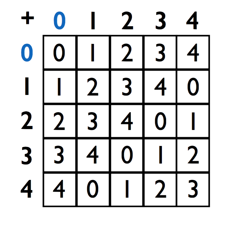
In $\mathbb Z_N$ , the element 0 is called the additive identity. It has the property that for any $A \in \mathbb Z_N$ , $A +_N 0 = 0 +_N A = A$ .

Exercise (Addition modulo

N

behaves nicely)

Show that if $A \equiv_N B$ and $A' \equiv_N B'$ , then $A+ A' \equiv_N B+B'$ .
Show that for any $A,B \in \mathbb Z$ , $(A + B) \bmod N = (A \bmod N) +_N (B \bmod N).$

Definition (Additive inverse)

Let $A \in \mathbb Z_N$ . The additive inverse of $A$ , denoted $-A$ , is defined to be an element in $\mathbb Z_N$ such that $A +_N -A = 0$ .

Exercise (Additive inverses modulo

N

are unique)

Show that every element of $\mathbb Z_N$ has a unique additive inverse.

Definition (Subtraction in

\mathbb Z_N

)

Let $A, B \in \mathbb Z_N$ . We define “ $A$ minus $B$ ”, denoted $A -_N B$ , as $A +_N -B$ .

Exercise (Addition table permutation property)

Show that in the addition table of $\mathbb Z_N$ , every row and column is a permutation of the elements $\mathbb Z_N$ .

Definition (Multiplication in

\mathbb Z_N

)

For $A, B \in \mathbb Z_N$ , we define the multiplication of $A$ and $B$ , denoted $A \cdot_N B$ , as $AB \bmod N$ . If $N$ is clear from the context, we can drop the subscript $N$ from $\cdot_N$ and write $\cdot$ . Furthermore, we can even drop $\cdot$ and represent $A \cdot_N B$ as simply $AB$ .

Exercise (Multiplication modulo

N

behaves nicely)

Show that if $A \equiv_N B$ and $A' \equiv_N B'$ , then $AA' \equiv_N BB'$ .
Show that for any $A,B \in \mathbb Z$ , $AB \bmod N = (A \bmod N) \cdot_N (B \bmod N).$

Definition (Multiplicative inverse)

Let $A \in \mathbb Z_N$ . The multiplicative inverse of $A$ , denoted $A^{-1}$ , is defined to be an element in $\mathbb Z_N$ such that $A \cdot_N A^{-1} = 1$ .

Proposition (Multiplicative inverse characterization)

Let $A,N \in \mathbb N$ . The multiplicative inverse of $A$ in $\mathbb Z_N$ exists if and only if $\gcd(A,N) = 1$ .

Definition (Division in

\mathbb Z_N

)

Let $A, B \in \mathbb Z_N$ , where $B$ has a multiplicative inverse $B^{-1}$ . Then we define “ $A$ divided by $B$ ”, denoted $A /_N B$ , as $A \cdot_N B^{-1}$ .

Definition (

\mathbb Z_N^*

)

We let $\mathbb Z_N^*$ denote the set $\{A \in \mathbb Z_N : \gcd(A, N) = 1\}$ . In other words, $\mathbb Z_N^*$ is the set of all elements of $\mathbb Z_N$ that have a multiplicative inverse.

Exercise (

\mathbb Z_N^*

is closed under multiplication)

Show that $\mathbb Z_N^*$ is closed under multiplication, i.e., $A,B \in \mathbb Z_N^* \implies A \cdot_N B \in \mathbb Z_N^*$ .

Note (Multiplication table for

\mathbb Z_N^*

)

Similar to an addition table for $\mathbb Z_N$ , one can consider a multiplication table for $\mathbb Z_N^*$ . For example, $\mathbb Z_8^* = \{1, 3, 5, 7\}$ , and the multiplication table is as below:

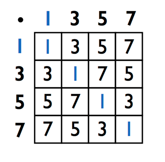
Exercise (Multiplication table permutation property)

Show that in the multiplication table of $\mathbb Z_N^*$ , every row and column is a permutation of the elements $\mathbb Z_N^*$ .

Definition (Euler totient function)

The Euler totient function $\varphi : \mathbb N\to \mathbb N$ is defined as $\varphi(N) = |\mathbb Z_N^*|$ . By convention, $\varphi(0) = 0$ .

Exercise (

\varphi(P)

and

\varphi(PQ)

)

Show that for $P$ a prime number, $\varphi(P) = P-1$ . Also show that for $P$ and $Q$ distinct prime numbers, $\varphi(PQ) = (P-1)(Q-1)$ .

Definition (Exponentiation in

\mathbb Z_N

)

Let $A \in \mathbb Z_N$ and $E \in \mathbb Z$ . We write $A^E$ to denote $\underbrace{A \cdot_N A \cdot_N \cdots \cdot_N A}_{E \text{ times}}.$

Theorem (Euler’s Theorem)

For any $A \in \mathbb Z_N^*$ , $A^{\varphi(N)} = 1$ . Equivalently, for any $A,N \in \mathbb Z$ with $\gcd(A,N) = 1$ , $A^{\varphi(N)} \equiv_N 1$ .

Note (Fermat’s Little Theorem)

When $N$ is a prime number, then Euler’s Theorem is known as Fermat’s Little Theorem.

Exercise (Reducing exponent modulo

\varphi(N)

)

Let $A \in \mathbb Z_N^*$ and $E \in \mathbb Z$ . Show that $A^E \equiv_N A^{E \bmod \varphi(N)}$ .

Exercise (Modular computation by hand)

Compute by hand $102^{98} \bmod 7$ .

Important Note (Exponent lives in

\mathbb Z_{\varphi(N)}

)

What the previous two exercises demonstrate is that if we are exponentiating an element $A \in \mathbb Z_N^*$ , then we can effectively think of the exponent as living in the set $\mathbb Z_{\varphi(N)}$ . This will be important to keep in mind when we cover Cryptography later.

Definition (Generator in

\mathbb Z_N^*

)

Let $A \in \mathbb Z_N^*$ . We say that $A$ is a generator if $\{A^E : E \in \mathbb Z_{\varphi(N)}\} = \mathbb Z_N^*.$

Theorem (

\mathbb Z_P^*

contains a generator)

If $P$ is a prime number, then $\mathbb Z_P^*$ contains a generator.

3. Modular operations: Computational complexity

Algorithm (Euclid’s gcd algorithm)

$\gcd(A, B)$ :

If $B = 0$ , then return $A$ .
Else return $\gcd(B, A \bmod B)$ .

Exercise (gcd property)

Show that if $A \geq B$ , $\gcd(A,B) = \gcd(A-B, B)$ . Use this to show that Euclid’s Algorithm correctly computes the greatest common divisor of two numbers.

Exercise (Time complexity of Euclid’s algorithm)

Suppose $A$ and $B$ can be represented with at most $n$ bits each. Give an upper bound on the number of recursive calls Euclid’s Algorithm makes in terms of $n$ .

Definition (Miix)

Let $A,B,C \in \mathbb N$ . We say that $C$ is a miix of $A$ and $B$ if $C = k A + \ell B$ for some $k, \ell \in \mathbb Z$ .

Exercise (Miix vs gcd 1)

Let $A,B,C \in \mathbb N$ . Show that if $C$ is a miix of $A$ and $B$ then $C$ is a multiple of $\gcd(A,B)$ .

Exercise (Miix vs gcd 2)

Show how to extend Euclid’s algorithm so that it outputs $k$ and $\ell$ such that $\gcd(A,B) = k A + \ell B$ . Then conclude that if $C$ is any multiple of $\gcd(A,B)$ , then $C$ is a miix of $A$ and $B$ .

Exercise

Prove Proposition (Multiplicative inverse characterization) using the previous two exercises.

Algorithm (Fast modular exponentiation)

$\text{FME}(A, E, N)$ :

Repeatedly square $A$ to obtain
$A^2 \bmod N$ , $A^4 \bmod N$ , $A^8 \bmod N$ , $\ldots$ , $A^{2^n} \bmod N$ .
Multiply together (modulo $N$ ) the powers of $A$ so that the product is $A^E$ .
To figure out which powers to multiply, look at the binary representation of $E$ .

Exercise

Suppose $A, E$ and $N$ are integers that can be represented using at most $n$ bits. Give an upper bound on the running time of the above algorithm in terms of $n$ .

4. Check Your Understanding

Problem

Wilson’s theorem states that $N$ is prime if and only if $(N-1)! \equiv_N N-1$ . Can we use this fact in the obvious way to design a polynomial time algorithm for isPrime?
True or false: Suppose that $A^K \equiv_N 1$ , where $A \neq 1$ . Then $\varphi(N) | K$ .
Determine, with proof, $750^{10002} \pmod{251}$ . Note that $251$ is prime.
Determine, with proof, $251^{(15^{251})} \pmod{7}$ .
Let $G$ be a generator in $\mathbb Z_N^*$ , and let $R \in \mathbb Z_{\varphi(N)}$ be chosen uniformly at random. For every $A \in \mathbb Z_N^*$ , determine $\Pr[G^R = A]$ .
Let $R \in \mathbb Z_N^*$ be chosen uniformly at random. For every $A, B \in \mathbb Z_N^*$ , determine $\Pr[A \cdot_N R = B]$ .
What is Euler’s Theorem?
What is a generator in $\mathbb Z_N^*$ ?
Consider the addition, subtraction, multiplication, division, exponentiation, taking logarithm, and taking root. Which of these operations are known to be polynomial-time solvable when the universe is the integers? Which of them are known to be polynomial-time solvable in the modular universe?
What is an efficient algorithm for finding the multiplicative inverse of an element in $\mathbb Z_N^*$ ?

5. High-Order Bits

Important Note

The theory behind modular arithmetic should mostly be review. It is important to know how the basic operations are defined and what kind of properties they have.
For which modular arithmetic operations do we have an efficient algorithm for (and what is that algorithm)? For which operations do we not expect to have an efficient algorithm? And for these operations, why don’t the “obvious” algorithms work? You should have a solid understanding of all these. Please internalize Important Note (Our model when measuring running time) and Important Note (Integer inputs are large numbers).

Cryptography

1. Private-key cryptographic system

Exercise (One-time pad based on modular multiplication)

Note that in the one-time pad cryptographic scheme described above, the underlying universe that we are dealing with is $\mathbb Z_2^n$ with the operation being bit-wise xor. Describe a similar scheme that uses $\mathbb Z_N^*$ as the universe.

2. Public-key cryptographic system

3. Check Your Understanding

Problem

Consider the one-time pad cryptographic system. Show that for any plaintext $M \in \{0,1\}^n$ , if the key $K \in \{0,1\}^n$ is chosen uniformly at random, then the ciphertext $C$ is a uniformly random element of $\{0,1\}^n$ .
Describe the Diffie-Hellman secret key exchange protocol.
Quantum computers can compute the discrete log problem efficiently. Explain how quantum computers can be used to break the Diffie-Hellman secret key exchange protocol.
Describe the RSA public-key protocol.
Quantum computers can compute the discrete root problem efficiently. Explain how quantum computers can be used to break the RSA public-key protocol.
Quantum computers can compute the factoring problem (given an integer $N$ , output its prime factors) efficiently. Explain how quantum computers can be used to break the RSA public-key protocol.

4. High-Order Bits

Important Note

Understand the general outline of how private-key protocols and public-key protocols work, independent of specific implementations of these ideas.
Make sure you understand how the one-time pad private-key protocol works and why it is a perfectly secure protocol.
You should be able to describe the Diffie-Hellman secret key exchange protocol and how it relates to the assumed hardness of the discrete log problem.
You should be able to describe the RSA public-key protocol and how it relates to the assumed hardness of the discrete root problem. You should also understand the relevance of the factoring problem in this setting.

Filters

Statement

Definition

Note

Question

Clear

Text

Overview